Optimizing Re-Chlorination Injection Points for Water Supply Networks Using Harmony Search Algorithm

1
Department of Civil Engineering, The University of Suwon, Gyeonggi-do 18323, Korea
2
K-Water, 200, Sintanjin-ro, Daedeok-gu, Daegeon 34350, Korea
3
Research Center for Disaster Prevention Science and Technology, Korea University, Seoul 02841, Korea
4
Department of Civil, Environmental and Architectural Engineering, Korea University, Seoul 02841, Korea
5
School of Civil, Environmental and Architectural Engineering, Korea University, Anam-ro 145, Seongbuk-gu, Seoul 02841, Korea
*
Author to whom correspondence should be addressed.
Water 2018, 10(5), 547; https://doi.org/10.3390/w10050547
Submission received: 16 March 2018
/
Revised: 16 April 2018
/
Accepted: 23 April 2018
/
Published: 25 April 2018
(This article belongs to the Special Issue Water Networks Management: New Perspectives)
Abstract
:In order to achieve the required residual chlorine concentration at the end of a water network, the installation of a re-chlorination facility for a high-quality water supply system is necessary. In this study, the optimal re-chlorination facility locations and doses were determined for real water supply systems, which require maintenance in ord3r to ensure proper residual chlorine concentrations at the pipeline under the present and future conditions. The harmony search algorithm (HSA), which is a meta-heuristic optimization technique, was used for the optimization model. This method was applied to two water supply systems in South Korea and was verified through case studies using different numbers of re-chlorination points. The results show that the proposed model can be used as an efficient water quality analysis and decision making tool, which showed the optimal re-chlorination dose and little deviation in the spatial distribution. In addition, the HSA results are superior to those of the genetic algorithm (GA) in terms of the total injection mass with the same number of evaluations.
1. Introduction
A water distribution network (WDN) is a critical civil infrastructure that supplies purified water to consumers. This purified water must be supplied in adequate quantities, at an adequate pressure, at an acceptable quality, and at affordable or socially fair prices that are based on the full water cost recovery principle [1,2]. When considering this, when an expanded water supply and a formation of district areas are required by a new town or large-scale residential complex construction, hydraulic and water quality modeling are essential to review the probability of a sufficient water supply and adequate residual chlorine. In particular, the maintenance of residual chlorine concentrations within a particular range is necessary to suppress microbial growth during water supply processes and to prevent the occurrence of diseases (e.g., diarrhoeal) that could be attributed to cross-contamination between the municipal water supply and sewer, due to leaky pipes, a lack of water pressure, and operational failures [3,4,5,6].
Studies related to the maintenance of residual chlorine concentrations within a particular range started by minimizing the mass of the disinfectant at the previously planned chlorine injection facilities. Boccelli et al. [7] performed a water quality analysis of a WDN using the primary reduction reaction of chlorine, which was used to minimize the amount of disinfectant that was injected at the previously determined re-chlorination points. It was found that low doses of chlorine disinfectant could adequately achieve quality standards when compared to traditional injection methods for the water source. In order to minimize the residual chlorine concentrations at the previously determined re-chlorination injection points, Munavalli and Kumar [8] studied the optimal chlorine concentration injection using a genetic algorithm (GA). Tryby et al. [9] and Lansey et al. [10] developed and used a mixed integer linear programming (MILP) model to determine the minimal disinfectant injection points. Gonelas et al. [5] suggested forming method for district metered areas (DMAs) while considering the chlorine residual concentration as the design criterion to minimize the highest cumulative sum of the chlorine residual in the network at any given time step. They applied their own optimization algorithms to minimize the operation pressure and chlorine residual concentration.
With respect to studies on the operation and maintenance of re-chlorination injection facilities, Propato and Uber [11] proposed an operation method that allows for the sums of the squared deviations of the residual concentrations to be minimized, in which the linear least-squares (LLS) optimization model was used. Ostfeld and Salomons [12] attempted to simultaneously optimize the pump operation and the re-chlorination injection facilities by combining a water quality simulation model with a GA, in which the operation and construction costs were used as the objective functions.
Prasad et al. [13] studied the booster facility location and injection-scheduling problem. They formulated a multi-purpose optimization that minimized the total disinfection dose while simultaneously maximizing the volume of water supplied to solve that particular problem. A multi-objective GA was used for that purpose. Islam et al. [14] proposed a water quality index (WQI) as a method to maintain an adequate residual chlorine level. This WQI is an overall index that considers the combined microbial, chemical, and aesthetic quality. Optimal re-chlorination injection points and amounts were determined based on the WQI. The proposed scheme was applied to the WDN for the city of Kelowna in British Columbia, Canada.
Recently, the disinfection by-products (DBPs) that were produced from the reaction between the disinfectant that was used for drinking water purification and the organic compounds in the water have been studied to comprehensively consider the factors for determining the re-chlorination injection points and facility operation scheme. Behzadian et al. [15] studied the formation reaction of trihalomethane (THM), which is one of the DBPs. They adopted a two-phase approach using a multi-purpose optimization technique. The booster chlorination operational injection cost (BCI) and booster chlorination capital cost (BCD) were used as the objective functions. The standard range of the THM concentration, a GA, and EPANET Multi-Species Extension (EPANET-MSX, [16]) were used as the constraint, optimization technique, and hydraulic analysis tool, respectively. Recently, Karadirek et al. [17] presented the application results for the management of the chlorine dosing rates in a real water distribution network, the Konyaalti water distribution network in Antalya, Turkey, using continuous monitoring and modeling techniques. Previous studies primarily used hypothetical distribution networks, with very few actual WDN case studies being reported. Furthermore, the optimization techniques that are typically applied are limited to the MILP model and GA.
In South Korea, the leakage ratio (real losses, as defined by IWA water loss task force [18] of water supply systems reached an average value of 15% [19]). Recently, WDNs have been evolving from branch-type into loop-type networks in order to decrease the leakage ratio during the supply process, improve the water quality, and to ensure a stable supply. However, branch-type networks remain in place in many regions of Korea. Because of these branch-type WDNs in Korea and the volatility of the chlorine disinfectant, high concentrations of residual chlorine are found in areas near the water purification plant where chlorine disinfection is carried out, while lower concentrations of residual chlorine are detected at the end trap of the pipe. The water quality standard for the residual chlorine in tap water in Korea ranges from 0.1 to 4.0 mg/L [20].
Thus, the purpose of this study was to solve an actual problem, which requires the installation of a re-chlorination injection facility. The harmony search algorithm (HSA), which is one of the latest meta-heuristic optimization models, is used to provide more accurate and reasonable results.
2. Problem Statements
2.1. Case Study Network 1
2.1.1. Network Description
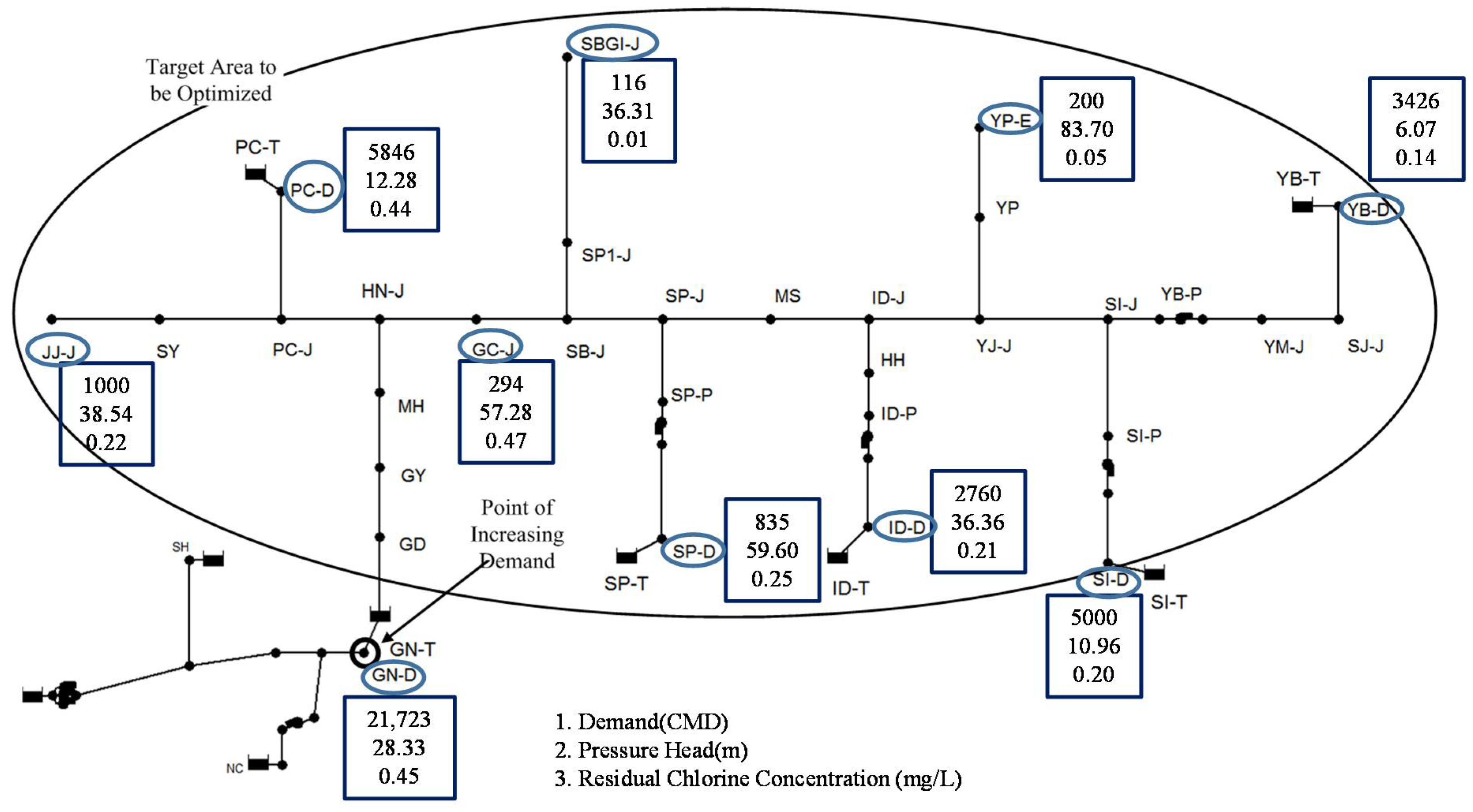
This study considered the WDN of P-City, in Korea, as the region for a case study. P-City covers an area of 826 km2 and it has a population of 119,750 water consumers. The water supply system of P-City includes approximately 85 km of water transportation pipes and 773 km of water distribution pipes. A total of eight distribution reservoirs supply 54,020 cubic meters per day (CMD) of water to the city. Figure 1 presents the configuration of the water transmission pipes in P-City.
2.1.2. Future Condition
P-City predicts an additional water demand of 10,000 CMD at site GN-D (circled in Figure 1), which is attributed to future water intake source changes and urban development. For such an additional water supply, the probability of a sufficient water supply and adequate residual chlorine must be verified using hydraulic and water quality modeling. The standard requires a concentration higher than 0.1 mg/L of residual chlorine for tap water, while for cases of contamination by potentially dangerous microscopic organisms e.g., Legionella and Mycobacterium avium [3,4], the residual chlorine concentration should be higher than 0.4 mg/L. For this reason, the P-City WDN manager plans to install a re-chlorination facility downstream of the GN-D point in order to maintain the residual chlorine concentration within the range of approximately 0.4 mg/L to 4.0 mg/L, even under additional water supply demand conditions.
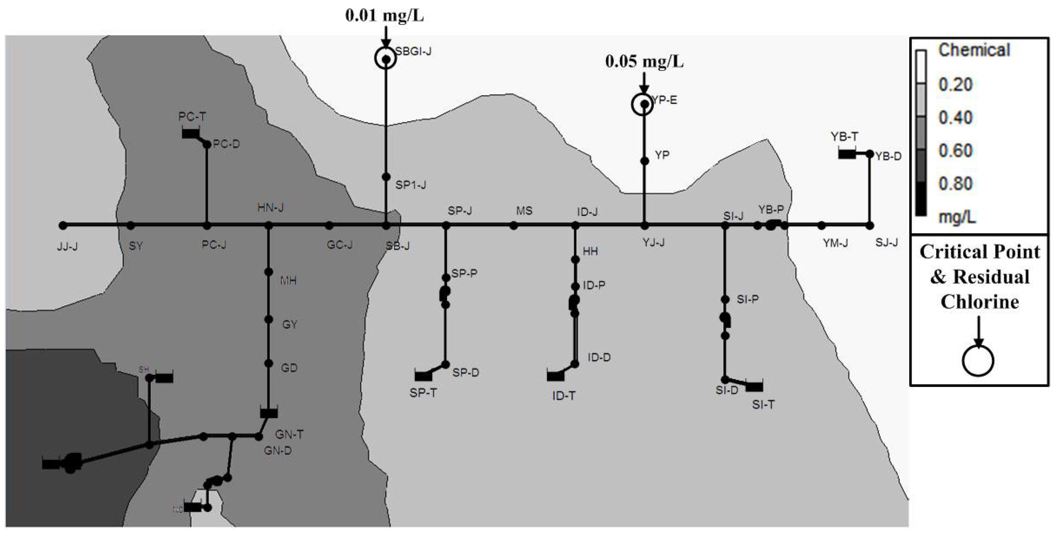
Figure 1 and Table 1 present the results of hydraulic and water quality analyses for the base scenario, in which the present chlorine injection points and amounts are maintained. The simulation results for the additional water supply include 21 nodes that do not meet the lower limit of 0.4 mg/L that is set by the water quality standards that were adopted. In the cases of YP-E and SBGI-J (critical points in Figure 2), which show higher retention times, the predicted values are 0.05 mg/L and 0.01 mg/L, respectively, which do not satisfy the lower limit of the regulatory standards. The average concentration of residual chlorine at the main nodes is 0.30 mg/L, which is also below the lower limits of the regulatory standards. Figure 2 presents the predicted spatial distribution of the residual chlorine concentrations. Thus, the water quality model that is based on the water demand data and present water pipeline of P-City suggests that the installation of a re-chlorination facility to ensure adequate residual chlorine concentrations is essential to ensure a stable water supply to faucets at the end of the pipeline.
2.2. Case Study Network 2
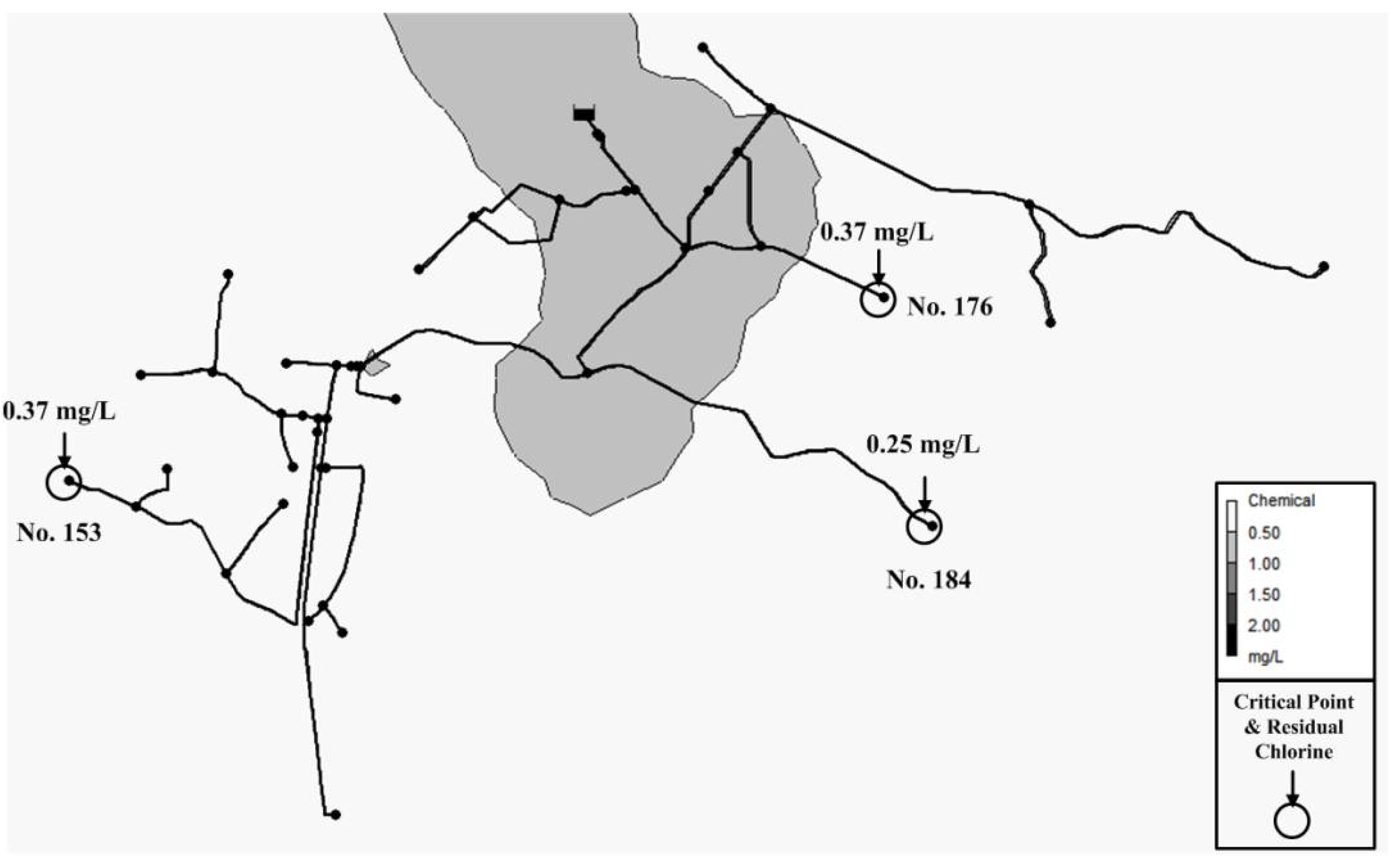
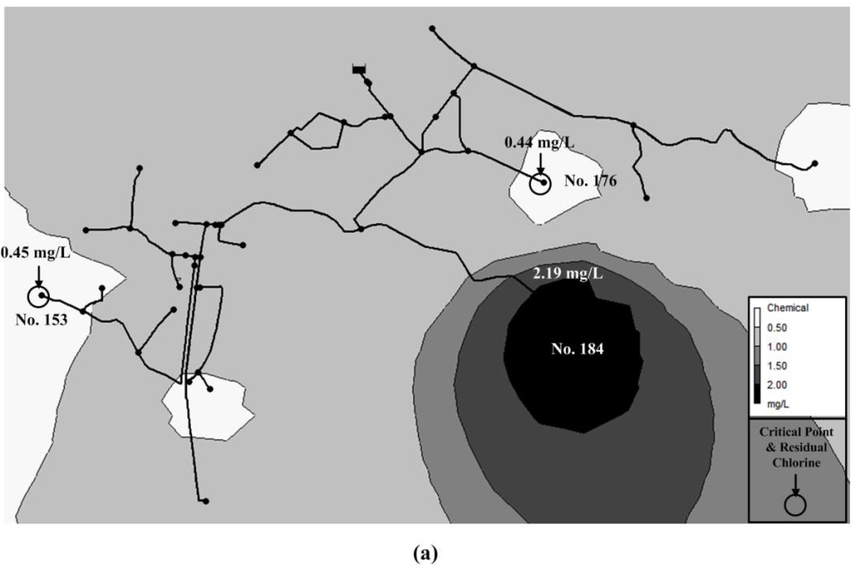
Network 2 is one of the small sub-areas in G-city that is covering an area of 517.2 km2 and having a population of 57,997 water consumers. The application region includes approximately 3.8 km of water distribution pipes. A small reservoir supplies 44 CMD. It consists of 47 distribution pipes and 45 water demand nodes. Figure 3 shows the configuration of the water distribution network in the target area. It shows the results of water quality analyses for the present conditions. The simulation results show that three demand nodes do not meet the lower limit of 0.4 mg/L. In the cases of nodes 153, 176, and 184 (critical points in Figure 3), the concentrations of residual chlorine are 0.37 mg/L, 0.37 mg/L, and 0.25 mg/L, respectively. These points are located at the end of the pipeline. Based on the present conditions, it is necessary to add re-chlorination injection facilities to ensure a stable water supply to the faucets at the end of the pipeline.
3. Model Formulation and Construction
In this section, the objective functions, decision variables, and constraints are formulated. The HSA results will be compared with those of the well-known GA. Therefore, the simulation process of HSA will be explained with the GA from the point of view of the methodology.
3.1. Objective Function and Constraints
The purpose of Equation (1) is to minimize the additional mass of disinfectant that will be injected into the WDN at specific predetermined nodes. The model decision variables are the booster injection mass rates for all of the nodes. The injection mass rate can be obtained by multiplying the booster injection concentration by the inflow rate for each node. Finally, the locations of the designed booster chlorination stations can also be determined.
Here, f denotes the total disinfectant dose (kg/d), Mi is the disinfectant mass (kg/d) at node i, and n represents the number of nodes.
There are four important constraints used in this optimization model. The first has to do with the concentration of residual chlorine at each node, which should range between the minimum and the maximum values (Equation (2)).
where Cli denotes the residual chlorine concentration at consumer node i (mg/L); Clmin and Clmax are the minimum and maximum residual chlorine requirements, respectively (mg/L); and, n denotes the number of nodes.
The second constraint has to do with the number of re-chlorination facilities to be installed. The number of re-chlorination facilities will be set as the preliminarily constraint in this model. Thus, various numbers of facilities will be set up for each scenario, and the optimization model will be simulated and analyzed.
where N denotes the number of re-chlorination facilities to be installed.
The two other constraints are hydraulic constraints, which are found using a hydraulic solver (EPANET [21] in this study). For each junction node, the mass conservation law should be satisfied, as shown in Equation (4).
where Qin and Qout are the flows into and out of the node, respectively; and, Qe is the external inflow rate or demand at the node.
For each loop in the network, the conservation of energy constraint should also be met.
where ∆Hk is the head loss in pipe k, and NL is the total number of loops in the system. The head loss in each pipe is the head difference between the connected nodes, and can be computed using the Hazen-Williams equation.
3.2. Harmony Search Algorithm for Solution Scheme Determination
The harmony search algorithm (HSA) that was proposed by Geem et al. [22] and Kim et al. [23] is an optimization method for finding a solution, just as an optimum chord or harmony in music is equivalent to the optimum solution in the field of engineering. When many different instruments play, the various sounds from each instrument generate a single chord. Out of all the chords, there will be an aesthetically pleasing one, but there may also be dissonance. The dissonance generated during the initial performance may gradually change to a suitable chord or harmony (local optimum), and finally reach an aesthetically pleasing chord or harmony (global optimum). In other words, the HSA is a technique in which the optimum harmony or chord searched for in music is the same as the optimum solution to be determined.
The HSA uses the harmony memory (HM), harmony memory considering rate (HMCR), pitch adjusting rate (PAR), and bandwidth (BW) as its main parameters. A memory space for each musician to remember the solutions is needed before starting the main process of the HSA, and a total harmony memory space where all of the memory spaces are gathered together will be generated. This is known as the HM, where the harmony memory size (HMS) represents the maximum number of harmonies to be saved in the memory space. Subsequently, the HSA will use three main operators: random selection (RS), memory consideration (MC), and pitch adjustment (PA), in order to seek better solutions (in terms of the objective function) from the previous HM.
The main steps of the HSA are summarized, as follows [24]:
Step 1: Generate random vectors (), as many as the HMS. Then, store these in the HM.
Step 2: Generate new harmonies. In generating a new harmony , for each component :
(Memory consideration, MC) With probability HMCR (0 ≤ HMCR ≤ 1), pick the stored value from the HM:
(Random selection, RS) With probability (1-HMCR), pick a random value within the range.
Step 3: Perform an additional process if the value in Step 2 came from the HM.
(Pitch adjustment, PA) With probability PAR (0 ≤ PAR ≤ 1), change by a small amount: for a continuous variable. BW is the amount of maximum change in pitch adjustment.
With probability (1-PAR), do nothing.
Step 4: Select the best harmonies, including new harmonies, as many as the HMS, and consider them to be the new HM matrix.
Step 5: Repeat from Step 2 to Step 4 until the termination criterion (e.g., the maximum number of function evaluations, iterations) is satisfied.
The HSA uses the HM, which is the set of aesthetically pleasing harmonies that are generated during the performance, and pleasing harmonies are saved at the same time in the memory space. Thus, the previous solutions are preserved using the memory space. The initial solutions used will be generated at random in order to avoid limiting them to a certain regional solution, and a neighboring solution will be generated during one iteration period. The HSA is a different search technique from the previous search techniques, such as simulated annealing (SA) and tabu search (TS). It has the same characteristic as TS, in that it enables a group search and contains cumulative previous experiences. At the same time, it has the same characteristic as SA, in that the solutions are added to the set of experiences if the solutions reach an acceptable range, even though they may not be optimal.
During the generation of a new solution using the GA, one of the best known meta-heuristic algorithms, only the two genes from the parents’ generation have an influence on the new gene, and only the parents’ experience becomes the information for the new gene. In contrast, the HSA acquires experience from all of the previous harmonies, because it uses improved solutions that were gained from previous iterations. This enables the determination of a new solution from a larger amount of information. One of the remarkable characteristics of the HSA, when compared with other algorithms, lies in the good harmony between an exploration/global search and the exploitation of the gained information/local search [25]. Algorithm 1 lists the general pseudo-code for the HSA.
The GA performs an exploitation/local search through the crossover of the parents’ solutions, and its exploration/global search can be executed by mutation (a change in a binary number, 1↔0). In other words, the exploitation/local search and exploration/global search are independently carried out using the GA. However, when the HSA generates a new harmony using the HMCR, it carries out the processes simultaneously, whether it uses the harmony in the HM (exploitation/local search) or it generates the harmony at random from the whole definition domain (exploration/global search). Even in the case of the PAR, it shows a unique performance in that both the exploitation and exploration processes progress in a harmonious manner, according to the bandwidth of the sound pitch.
| Algorithm 1 Pseudo-code for Harmony Search Algorithm (has) |
| Start Objective function f(M), M = (M1, M2, …, Mn)T (Mi is the disinfectant mass at node i, see Equation (1)) Generate initial harmonies (real number arrays candidate solution vectors) Define pitch adjusting rate (PAR), pitch limits (allowable disinfectant mass), and bandwidth (BW) Define harmony memory considering rate (HMCR) while (t < Max number of iterations) Generate new harmonics by accepting the best harmonies Adjust pitch to obtain new harmonies (solutions) if (rand > HMCR), choose an existing harmony randomly else if (rand < PAR), adjust the pitch randomly within the limits else generate new harmonies via randomization end if Calculate objective function and constraints check (see Equations (2)–(5)) of new harmonies Accept the new harmonies (solutions) if better end while Find the best current solution End |
3.3. Optimization Scheme and Flowchart
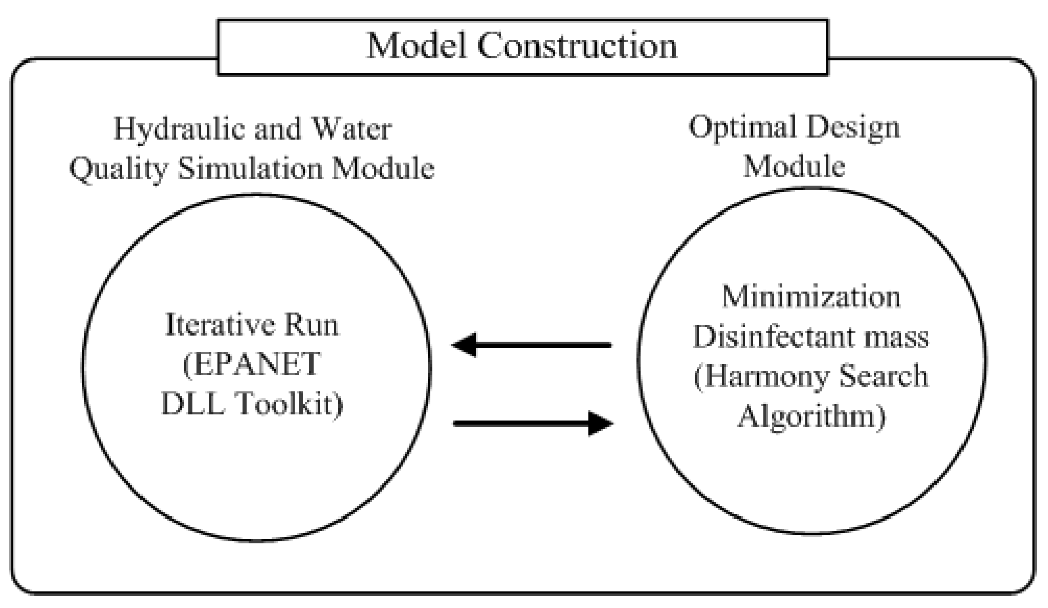
Figure 4 presents the components of the proposed model. The model is composed of two modules: the hydraulic and water quality simulation module and the optimal design module. The HSA, being one of the optimal design techniques, is used to calculate the optimal re-chlorination dose. It is necessary to review whether or not the water quality analysis results after re-chlorination meet the residual chlorine concentration constraint during the optimization process. In this regard, a repetitive hydraulic and quality analysis is needed, and the dynamic link library (DLL) toolkit from EPANET, which is one of the most widely used WDN analysis programs, is used.
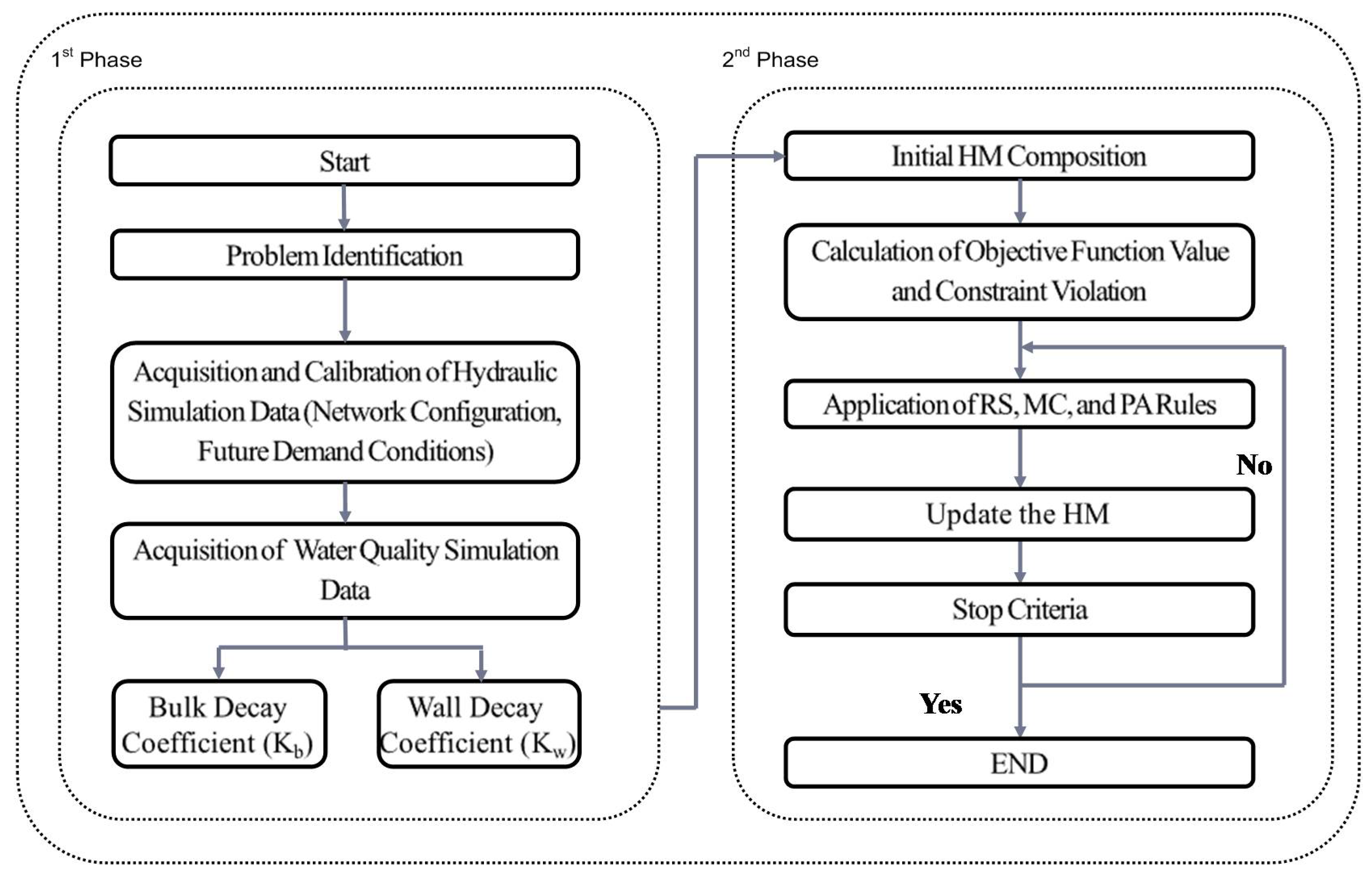
Two phases are required to simulate the proposed model (Figure 5). Phase 1 shows the composition of the input data for the operation of the optimization model, while phase 2 displays the optimization process flow. The details of each phase are summarized below.
The system must be operational to verify the constraints in phase 2. The pipeline network information is needed for the operation of EPANET. The current conditional data obtained through field surveys and water pressure/quality measurements are used for model calibration. The basic simulation data are then reviewed by considering the future demand conditions in this case study. In particular, the bulk decay coefficient (kb) and wall decay coefficient (kw) will be determined through laboratory experiments and the results of previous studies. These are the two main factors that are used in water quality analysis for determining the residual chlorine concentration as the constraint. The water quality parameters that are used here are shown in Section 4.1.
The process flow of the HSA for calculating the optimal re-chlorination will now be described. First, the sum of the re-chlorination doses to be injected into the nodes will be made equal to the number of the HMS. Because the number of re-chlorination injection points is initially fixed in this model, it is necessary to verify the set of HM and constitute an adequate HM that is equivalent to the number of re-chlorination points. The next step is to calculate the objective function of the first set of HM and to apply the penalty function to the HM according to the constraint violation. The solutions that violate the constraints will gradually be removed from the optimal solutions set through an iteration process. This process generates new solutions using the three operators of the HSA (RS, MC, and PA), and continuously saves better solutions through comparisons with the previous HM solutions. If the solutions meet the initially set termination condition, then the optimization process will terminate, and the final solutions will be printed out. This study used the maximum number of iterations as the termination condition.
4. Application Results
4.1. Applied Data and Scenarios
The chlorine decay models can be classified into a first-order decay model and a power-law decay (nth order) model, according to the order of the decay equation [26,27]. The factors that control the chlorine concentration in the pipe are the bulk decay reaction with the water constituents, and the wall decay reaction with the biofilm, wall materials, and tubercles. The first-order chlorine decay model for the bulk and wall decay is more popular and is generally accepted because of its simplicity and the availability of analytic solutions [28,29,30]. Thus, the first-order chlorine decay model, which considers the bulk and wall effects, is employed here.
This study used the experimental data produced by K-Water [31] as the water quality analysis parameters. They carried out a bottle test using a serum bottle (160 mL) and a Teflon-coated silicon cap to obtain the bulk decay coefficients with temperature change. The residual chlorine concentration was measured over time, after the injection of an initial chlorine concentration of 1 mg/L under different temperature conditions: 4.5 °C, 18 °C, and 25 °C. Because the residual chlorine concentration gradually decreases with the reaction time, the measurement interval is less than 24 h. After 24 h have passed, measurements are carried out for an additional 150 h (174 h in total) by increasing the interval. The measurement data are used in the Arrhenius equation (Equation (7)) to determine the decay coefficient correlation equations. The bulk decay coefficients in the pipeline have values of −0.0046, −0.0135, and −0.024 h−1, at temperatures of 4.5 °C, 18 °C, and 25 °C, respectively.
Here, k denotes the rate constant of the chemical reaction, T is the absolute temperature (in degrees Kelvin), A is the pre-exponential factor, Ea is the activation energy, and R is the universal gas constant.
If the change in bulk decay coefficient with temperature that was obtained from the experiment is plotted on a graph of versus the absolute temperature, a linear trend line is obtained, and the calculation of an estimation equation for the bulk decay coefficient with temperature may be carried out. In other words, the linearization of Equation (4) yields , where and are the constants. This produces a linear correlation between the temperature (T) and . Equation (8) presents the correlation between the bulk decay coefficient of the residual chlorine and the temperature.
Here, k denotes the rate constant of a chemical reaction, and T is the absolute temperature (in degrees Kelvin).
The final bulk decay coefficients in the pipeline are −0.1056, −0.1872, and −0.5760 d−1 at temperatures of 4.5 °C, 18 °C, and 25 °C, respectively. For a conservative approach, this study selected a value of −0.5760 d−1 for the bulk decay coefficient at 25 °C as the worst-case scenario. The value of −0.1 d−1 was selected as the wall decay coefficient, because it was recommended in previous studies [32,33]. The selection of this value was also based on the material of the construction, the present condition (in need of repair), and the age of the pipe.
The model for the optimal re-chlorination injection points and dose was simulated for the purpose of this study based on the data obtained from the hydraulic and water quality analyses of the WDN. In this study, the number of re-chlorination injection points was limited to two, three, and four points, as a constraint for the operation of the model.
4.2. Sensitivity Analysis of Parameters
A sensitivity analysis was performed to investigate the effects of the HSA parameter values (i.e., HMCR and PAR) on its performance. Various parameter sets were examined in order to find the optimal solutions for the P-City network. The HMCR value generally varies from 0.7 to 0.99 (typical value = 0.9). In the case of PAR, it generally varies from 0.1 to 0.5 (typical value = 0.3). Therefore, the available combinations of HMCR (0.7, 0.8, and 0.9) and PAR (0.1, 0.2, and 0.3) values (nine cases) were investigated in the sensitivity analysis. The HMS and BW values were set at 30 and 0.01, respectively, which are known to be the typical values [25].
Table 2 lists the rankings of the parameter combinations in terms of the solution quality for the two, three, and four injection point scenarios. As can be seen in Table 2, case 1 (HMCR = 0.7, PAR = 0.1) had the first total rank (sum rank) among the nine cases, providing a better optimal value (the total disinfectant dose). Therefore, the calculation of the optimal solutions using various parameter combinations showed the best results when the following combination was used: HMS = 30, HMCR = 0.7, PAR = 0.1, and BW = 0.01.
4.3. Application Results
4.3.1. Case Study Network 1
The calculation results for the optimal solutions were obtained by setting the number of re-chlorination injection points at two (scenario 1), three (scenario 2), and four (scenario 3). The locations of the re-chlorination points for the three scenarios that were determined by the optimization are shown in Figure 6. In the case of scenario 1, a larger re-chlorination dose is injected at the main branches that are located upstream from the network, since the installation is limited to only two points. In other words, the “degree of node” can also be utilized, which is defined as the number of pipes that are connected to a node, to explain the optimal results. As the number of links that are connected to a node increases, the available paths connecting water sources to nodes also increase. The “degree of node” of HN-J is three. This means that it has an advantage because it could have alternative paths and has higher connectivity than other nodes. The other re-chlorination facilities that are installed at the end of pipelines hardly meet the criteria for the minimum concentration of residual chlorine because of long retention times. For scenarios two and three, because the water flow in the pipeline is significant, the sum of the re-chlorination injections may be greatly decreased through optimization. An injection decrease is shown at the upstream nodes in the network, which require large injection amounts, whereas additional facilities for re-chlorination are installed in the middle of the network.
Table 3 lists the detail numerical results. The results for scenario 1 show that nodes HN-J and SBGI-J are in need of re-chlorination. In order to maintain the residual chlorine concentrations higher than 0.4 mg/L at nodes SBGI-J, and YP-E (critical points in Figure 2), it is necessary to increase the re-chlorination injection at nodes HN-J and SBGI-J to 3.31 mg/L and 2.47 mg/L, respectively. SBGI-J and YP-E are the nodes with low residual chlorine concentrations. The injection concentrations at nodes HN-J and SBGI-J can be converted into doses of 64.47 kg/d and 0.29 kg/d, respectively, which means that a total amount of 64.76 kg/d (optimal value) should be injected. The total re-chlorination dose increases as the water flow along the connection pipeline increases, even if the same concentration of re-chlorination is required. Therefore, node HN-J, which is located upstream from the water network, requires the highest re-chlorination dose. According to the water quality analysis, which uses the determined injection dose, the residual chlorine concentrations are in the range of 0.40 mg/L (minimum) to 3.80 mg/L (maximum).
Scenario 2 introduces one more re-chlorination node, YP, which is added to the previous two nodes (HN-J and SBGI-J) that were selected for scenario 1. In order to maintain a residual chlorine concentration higher than 0.4 mg/L, which is the minimum for the water network, it is necessary to increase the re-chlorination injections at HN-J, SBGI-J, and YP to 1.20 mg/L, 3.59 mg/L, and 1.45 mg/L, respectively. Such injection concentrations can be converted into a total dose of 24.08 kg/d. When compared with scenario 1, the total dose to be injected at node HN-J, which is located upstream within the network, decreases to approximately one-third of the previous value. According to the water quality analysis using the determined injection dose, the residual chlorine concentrations are in the range of 0.45 mg/L (minimum) to 3.64 mg/L (maximum).
Scenario 3 introduces two more re-chlorination nodes, GD and SP-J, which are added to the previous two nodes (SBGI-J and YP) that are selected for scenario 2. In order to maintain a residual chlorine concentration that is higher than 0.4 mg/L, which is the minimum for the water network, it is necessary to increase the re-chlorination injections at GD, SP-J, SBGI-J, and YP to 110.91 kg/d, 8.19 kg/d, 0.16 kg/d, and 0.64 kg/d, respectively. The total injection dose amounts to 19.90 kg/d. Compared with scenario 2, the total dose to be injected at HN-J is approximately 4.18 kg/d lower than that for scenario 2. According to the water quality analysis using the determined injection dose, the residual chlorine concentrations are in the range of 0.43 mg/L (minimum) to 3.58 mg/L (maximum).
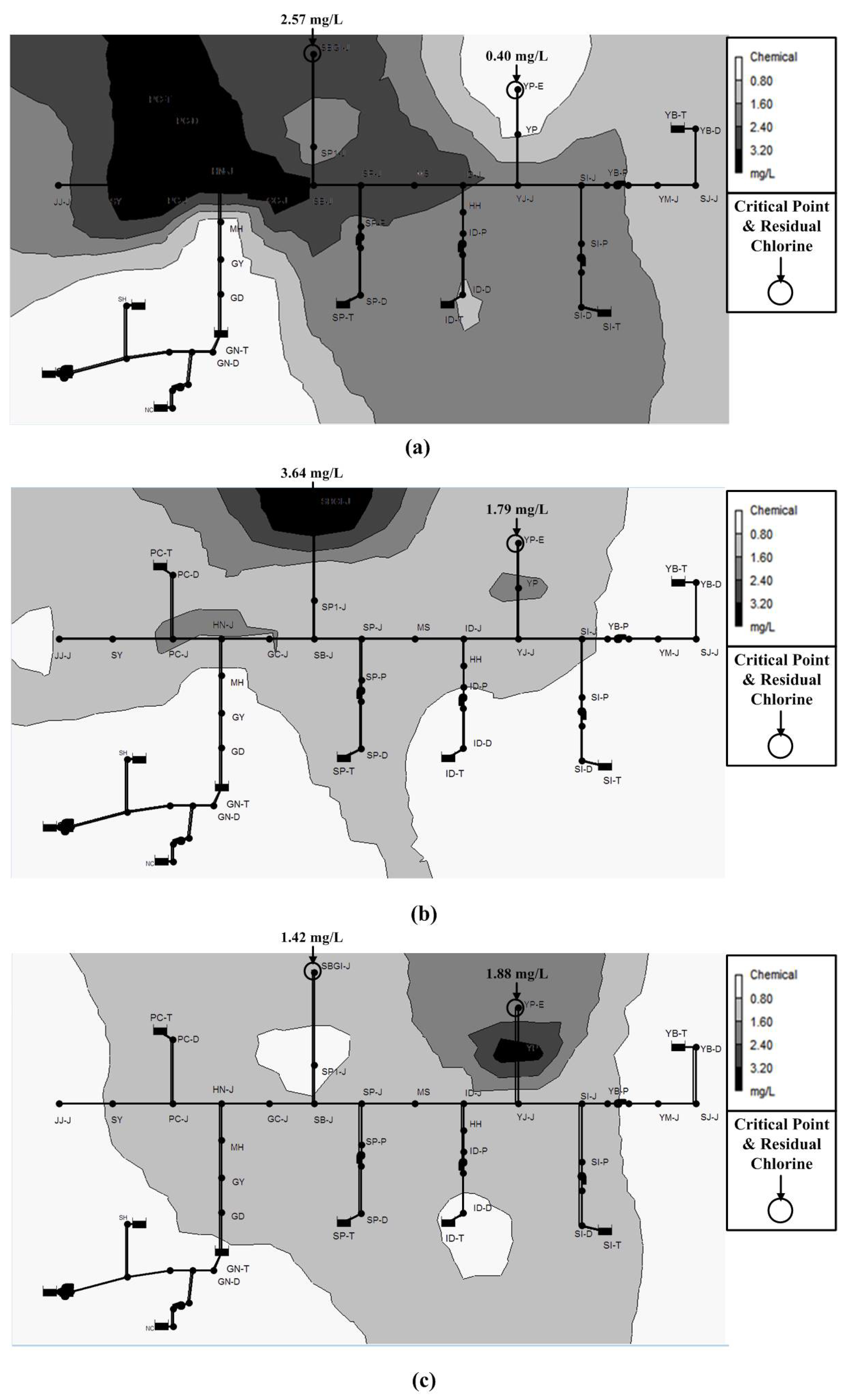
These three scenarios, with different numbers of re-chlorination points (two, three, and four) that are determined by the optimization results, prove that the operation schemes achieve the residual chlorine concentration (approximately 0.4–4.0 mg/L) quality standard. However, using high concentrations of residual chlorine may cause people to avoid drinking tap water. Consequently, it may also cause an increase in the concentration of DBPs. In this respect, it is advisable to lower the maximum and the average concentrations of residual chlorine, if possible, in the WDN. Figure 7 shows the residual chlorine concentration spatial distribution after the optimization of each scenario. The average concentrations of residual chlorine after the optimizations of each scenario are 1.96 mg/L, 1.06 mg/L, and 1.02 mg/L, respectively. The maximum concentrations are 3.80 mg/L, 3.64 mg/L, and 3.58 mg/L, respectively. As the number of re-chlorination points increases, the average and maximum concentrations of residual chlorine decrease. This means that increasing the number of re-chlorination points helps to maintain a low concentration and a low standard deviation of residual chlorine, and it also produces a flat water quality analysis spatial distribution.
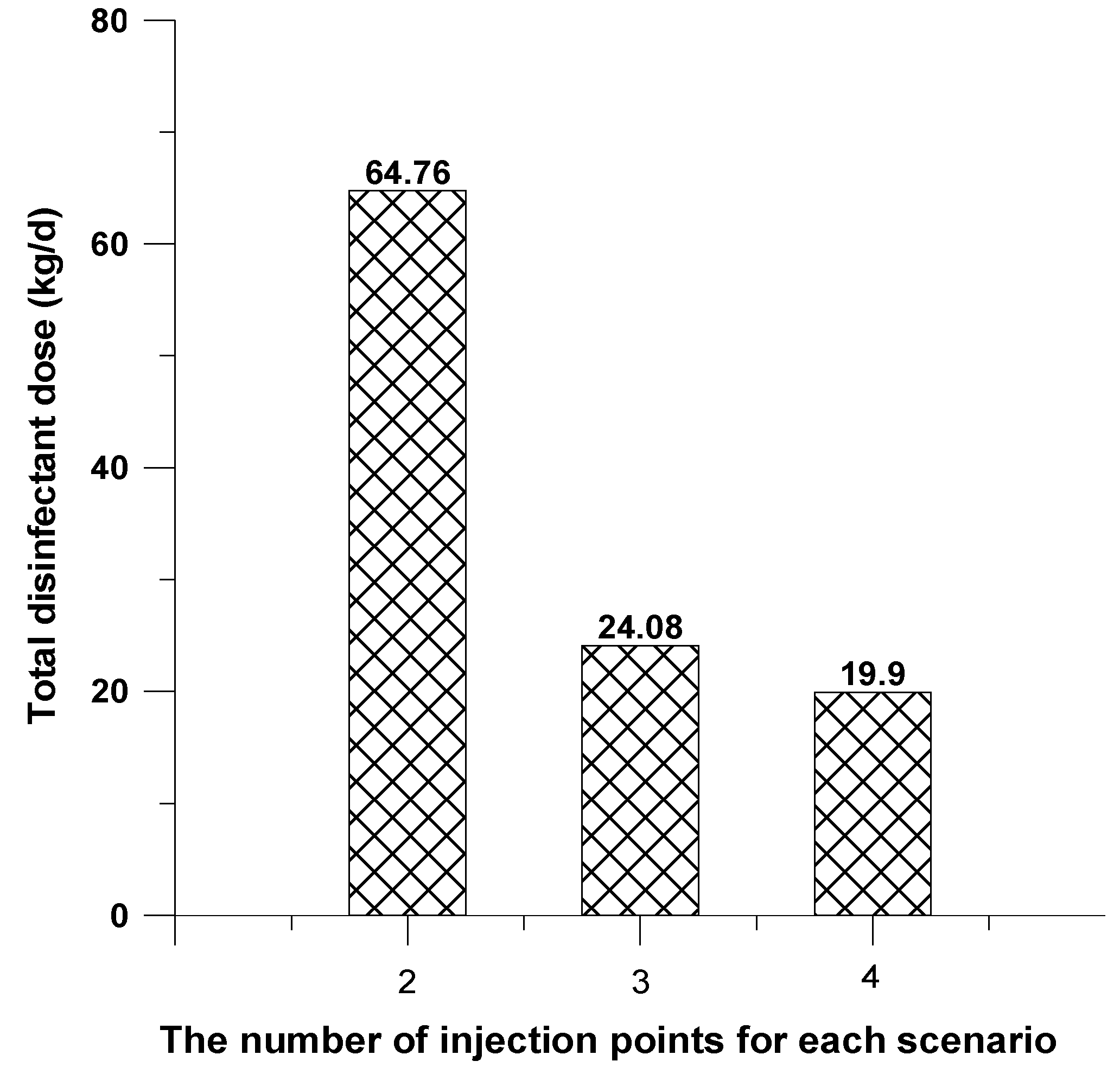
Figure 8 shows the total injection doses for the three scenarios with different numbers of injection points (two, three, and four points), as determined through the optimizations. Because scenario 1 must satisfy the residual chlorine level for the entire water network using only two re-chlorination injection points, a greater amount of re-chlorination is required. Meanwhile, one or two additional re-chlorination installation points (scenarios 2 and 3) allow for a decrease in the injection dose to one-third of that from scenario 1.
For comparison purposes, the optimization results that were obtained by two meta-heuristic algorithms (HSA and GA) are provided. In this comparison, the same initial population size (i.e., 30) as the HSA was considered for the GA. The initial parameters for the GA were a mutation rate of 0.1 and crossover rate of 0.7. To ensure a fair quantitative evaluation and judgment between the HSA and GA, the same number of functional evaluations (50,000) was used in this simulation.
As listed in Table 4, the HSA results are superior to those of the GA in terms of the total injection mass with the same number of evaluations.
4.3.2. Case Study Network 2
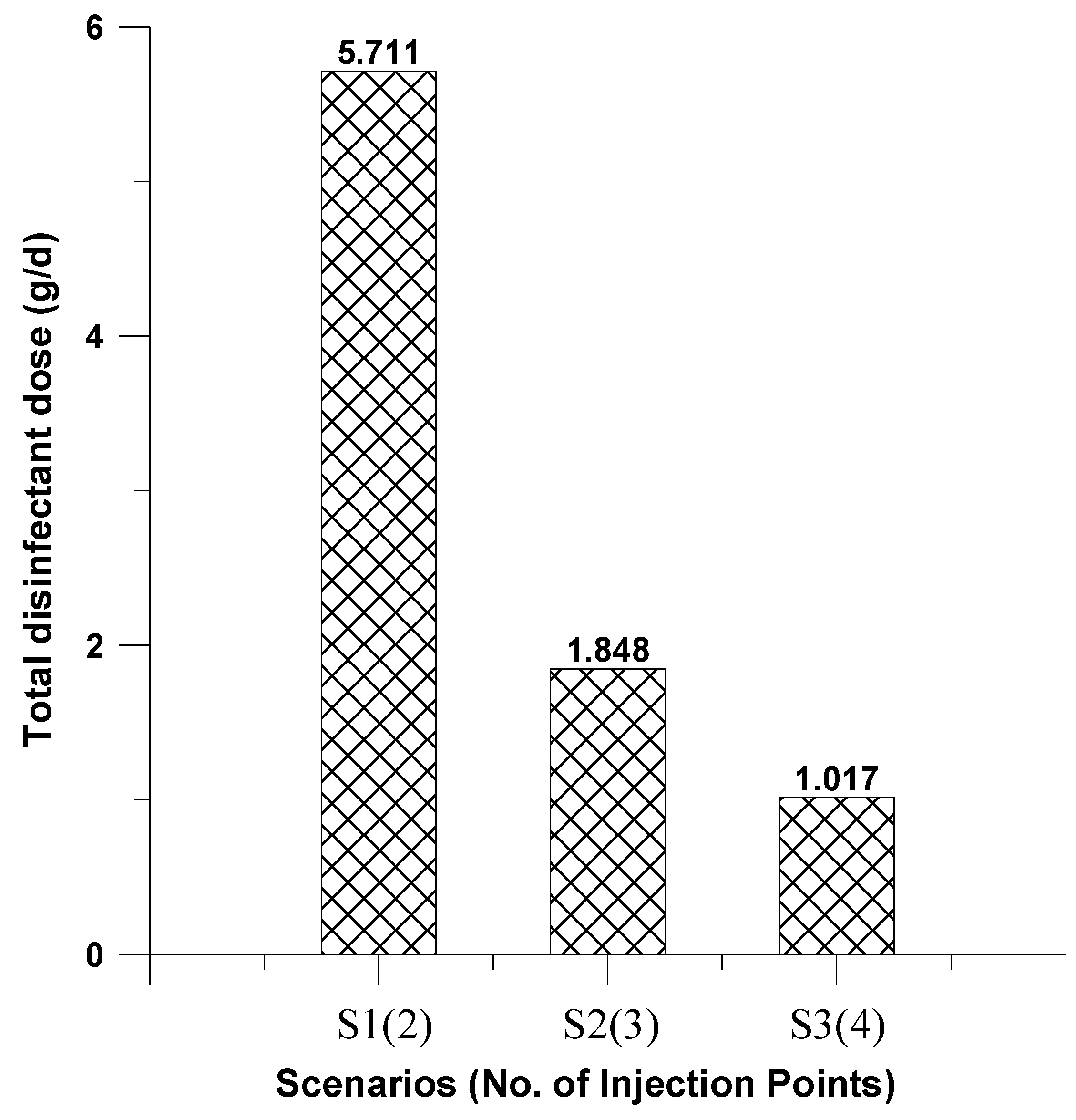
The calculation results for network 2 were also obtained by considering two (scenario 1), three (scenario 2), and four (scenario 3) re-chlorination injection points. Figure 9 shows the total injection doses for the three scenarios that were determined through optimization. Network 2 had results that were similar to network 1 (P-City). The total disinfectant dose was dramatically decreased when the number of re-chlorination injection points was changed from two to one. In other words, one or two additional re-chlorination installation points (scenarios 2 and 3) allow for a sharp decrease in the injection dose to about one-third of that from scenario 1.
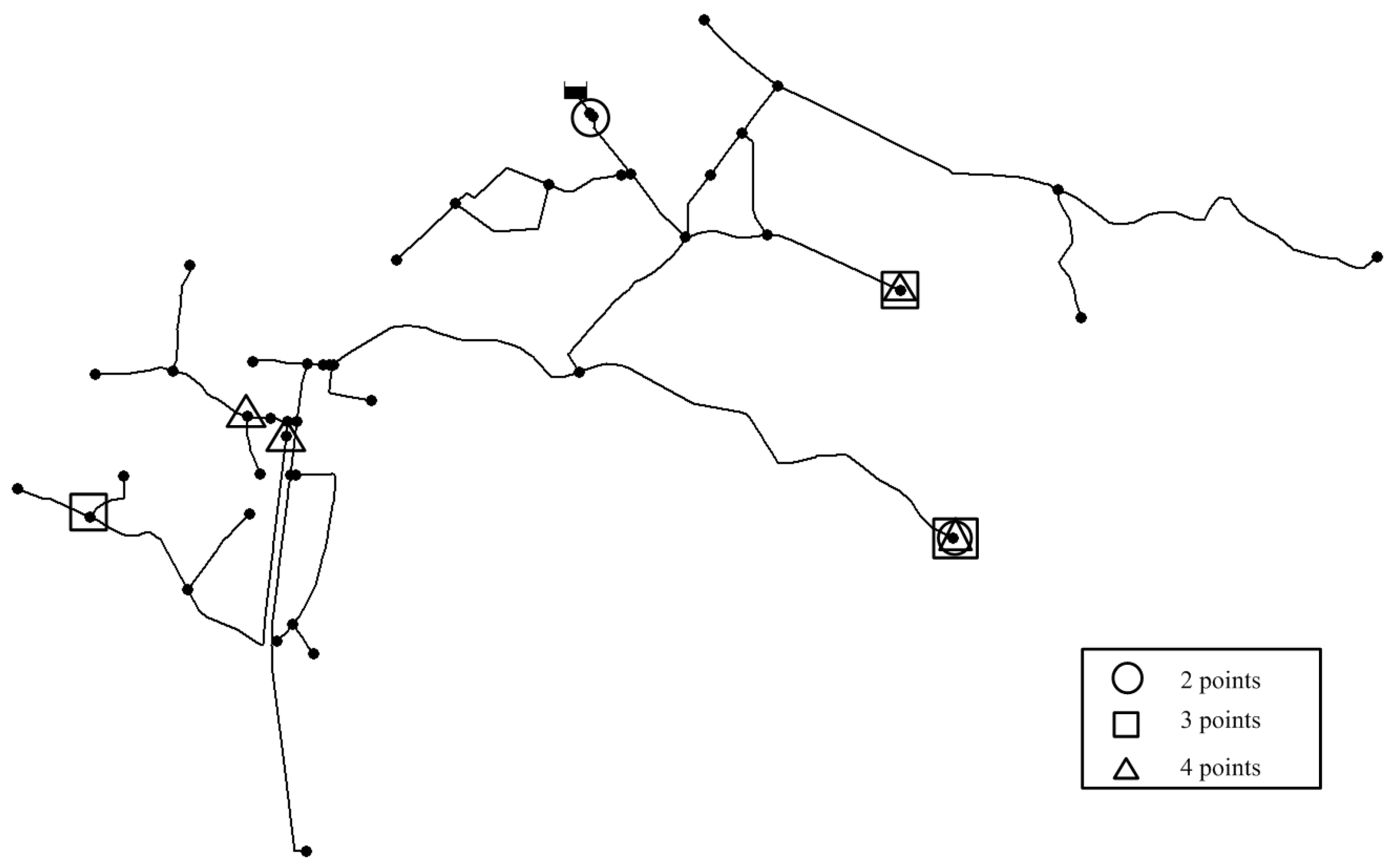
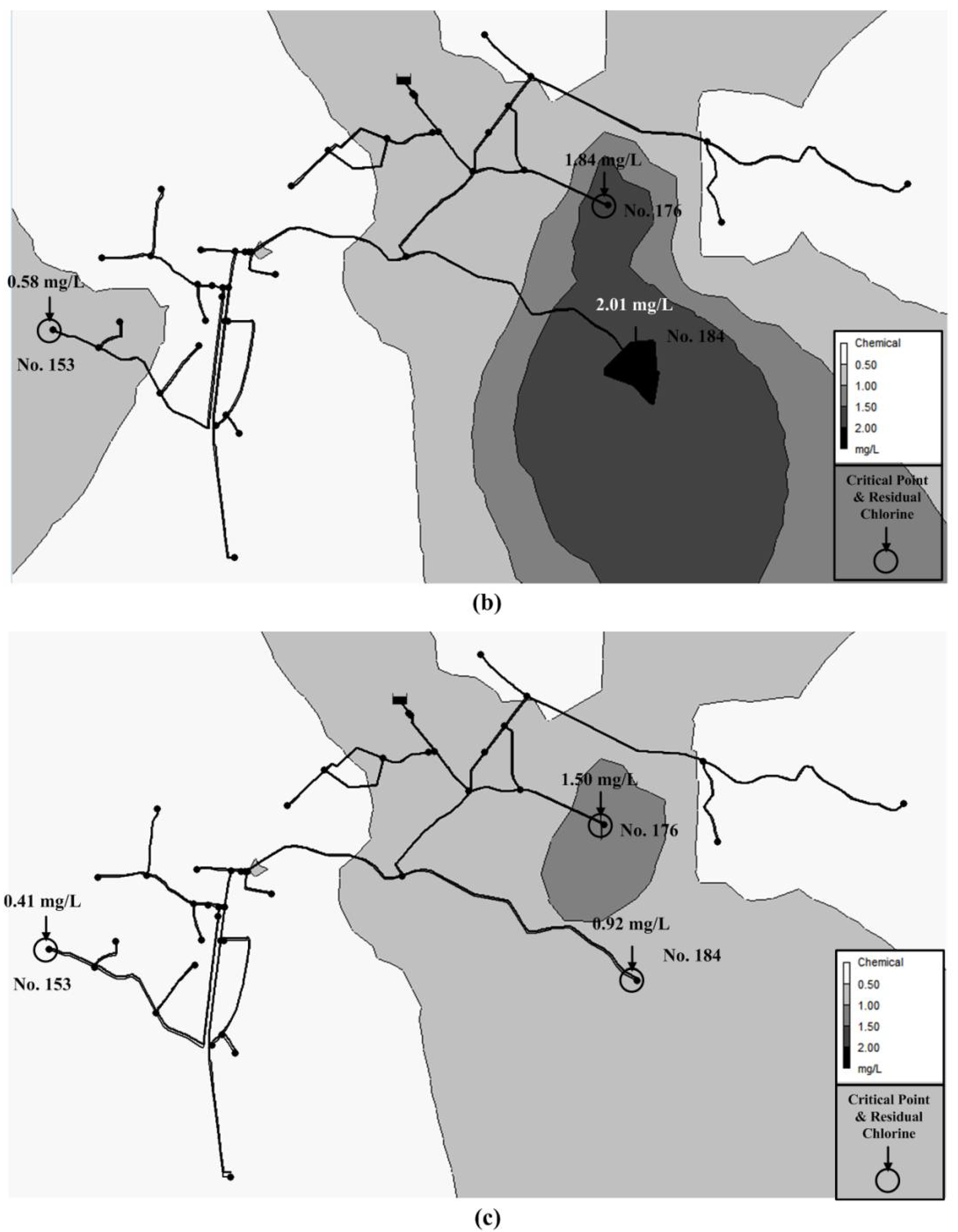
Figure 10 shows the locations of the re-chlorination points for the three scenarios, as determined by the optimization. In the case of scenario 1, a re-chlorination facility is installed at the node that is closest to the source, because the installation is limited to only two points. The other re-chlorination facilities are installed at the end of the pipeline (at one of the critical nodes in Figure 3). For scenarios 2 and 3, because the water flow in the pipeline is significant, the sum of the re-chlorination injections may be largely decreased through optimization. In relation to the location, the additional facilities for re-chlorination are installed in the middle of the network, which has a larger value for the “degree of node”. Figure 11 shows each scenario’s residual chlorine concentration spatial distribution after optimization. As the number of re-chlorination points increases, the maximum concentration of residual chlorine decreases.
5. Conclusions
An optimization model was proposed in this study to determine the re-chlorination facility locations and the doses for two real water supply networks (P-City and network 2), which require maintenance in order to ensure appropriate residual chlorine concentrations for faucets at the end of the pipeline under the present and future conditions. The HSA, which is a meta-heuristic optimization technique, was used for the optimization model in this study, and was simulated through case studies using different numbers of re-chlorination points (two, three, and four points). The optimization results satisfied the minimum and maximum concentration requirements for residual chlorine at all of the nodes. Because high concentrations of residual chlorine in the pipeline could cause an increase in DBPs, it is advisable to lower the maximum and average concentrations of residual chlorine, if possible, in the WDN. In addition, the HSA results are superior to those of the GA in terms of the total injection mass with the same number of evaluations.
The water flow in the pipeline decreased from upstream to downstream locations. If re-chlorination facilities are installed at an upstream location, then a large amount of re-chlorination injection is required in order to maintain a stable concentration of residual chlorine. In this regard, the re-chlorination locations and the doses of the nodes should be well distributed spatially in order to minimize the required injection quantity. In particular, if the re-chlorination facilities are installed at only one or two nodes upstream from the network, to satisfy the residual chlorine requirement at all of the nodes, the solution feasibility and efficiency decrease because the injection amount exponentially increases. This model presented an efficient water quality analysis, which showed the optimal re-chlorination dose and little deviation in the spatial distribution with the pre-determined number of re-chlorination points. An increase in the re-chlorination points made it simple to maintain a low residual chlorine concentration with little deviation, and it produced a flat spatial water quality analysis distribution. In this regard, the model proposed in this paper could be used as a decision-making tool for a stable water supply. Although optimization techniques have recently been applied to some hydraulic design parameters, such as the node pressure and pipe flow velocity, only trial-and-error-based techniques are currently used for water quality modeling. Therefore, this model will be useful for the design of new WDNs and the development of their operation and management guidelines.
Further study is required to achieve an optimal residual chlorine concentration over the entire time period of an extended simulation, rather than based on the average demand. In addition, it is necessary to further study multi-objective optimization by considering the economic feasibility in accordance with the installation and operation of re-chlorination facilities.
Author Contributions
Do Guen Yoo and Joong Hoon Kim conceived and designed the original idea of proposed method; Do Guen Yoo and Sang Myoung Lee carried out survey of previous studies; Do Guen Yoo, Ho Min Lee, and Young Hwan Choi analyzed the data; Do Guen Yoo wrote the paper.
Funding
This research was funded by [National Research Foundation of Korea] grant number [2016R1A2A1A05005306].
Acknowledgments
The study was supported by Korea Ministry of Environment as “Projects for Developing Eco-Innovation Technologies (2016002120004)”.
Conflicts of Interest
The authors declare no conflict of interest.
References
- Kanakoudis, V.; Tsitsifli, S. Socially fair domestic water pricing: Who is going to pay for the non-revenue water? Desalination Water Treat. 2016, 57, 11599–11609. [Google Scholar] [CrossRef]
- Tsitsifli, S.; Gonelas, K.; Papadopoulou, A.; Kanakoudis, V.; Kouziakis, C.; Lappos, S. Socially fair drinking water pricing considering the Full Water Cost recovery principle and the Non-Revenue Water related cost allocation to the end users. Desalination Water Treat. 2017, 99, 72–82. [Google Scholar] [CrossRef]
- World Health Organization (WHO). Safe Piped Water: Managing Microbial Water Quality in Piped Distribution Systems; Ainsworth, R., Ed.; IWA Publishing: London, UK, 2004. [Google Scholar]
- Payment, P.; Robertson, W. The microbiology of piped distribution systems and public health. In Safe Piped Water: Managing Microbial Water Quality in Piped Distribution Systems; IWA Publishing: London, UK, 2004; pp. 1–18. [Google Scholar]
- Gonelas, K.; Chondronasios, A.; Kanakoudis, V.; Patelis, M.; Korkana, P. Forming DMAs in a water distribution network considering the operating pressure and the chlorine residual concentration as the design parameters. J. Hydroinform. 2017, 19, 900–910. [Google Scholar] [CrossRef]
- Kanakoudis, V.; Tsitsifli, S. Potable water security assessment—A review on monitoring, modelling and optimization techniques, applied to water distribution networks. Desalination Water Treat. 2017, 99, 18–26. [Google Scholar] [CrossRef]
- Boccelli, D.L.; Tryby, M.E.; Uber, J.G.; Rossman, L.A.; Zierolf, M.L.; Polycarpou, M.M. Optimal scheduling of booster disinfection in water distribution systems. J. Water Resour. Plan. Manag. 1998, 124, 99–111. [Google Scholar] [CrossRef]
- Munavalli, G.R.; Kumar, M.M. Optimal scheduling of multiple chlorine sources in water distribution systems. J. Water Resour. Plan. Manag. 2003, 129, 493–504. [Google Scholar] [CrossRef]
- Tryby, M.E.; Boccelli, D.L.; Uber, J.G.; Rossman, L.A. Facility location model for booster disinfection of water supply networks. J. Water Resour. Plan. Manag. 2002, 128, 322–333. [Google Scholar] [CrossRef]
- Lansey, K.; Pasha, F.; Pool, S.; Elshorbagy, W.; Uber, J.G. Locating satellite booster disinfectant stations. J. Water Resour. Plan. Manag. 2007, 133, 372–376. [Google Scholar] [CrossRef]
- Propato, M.; Uber, J.G. Linear least-squares formulation for operation of booster disinfection systems. J. Water Resour. Plan. Manag. 2003, 130, 53–62. [Google Scholar] [CrossRef]
- Ostfeld, A.; Salomons, E. Conjunctive optimal scheduling of pumping and booster chlorine injections in water distribution systems. Eng. Optim. 2006, 38, 337–352. [Google Scholar] [CrossRef]
- Prasad, T.D.; Walters, G.A.; Savic, D.A. Booster disinfection of water supply networks: Multiobjective approach. J. Water Resour. Plan. Manag. 2004, 130, 367–376. [Google Scholar] [CrossRef]
- Islam, N.; Sadiq, R.; Rodriguez, M.J. Optimizing booster chlorination in water distribution networks: A water quality index approach. Environ. Monit. Assess. 2013, 185, 8035–8050. [Google Scholar] [CrossRef] [PubMed]
- Behzadian, K.; Alimohammadnejad, M.; Ardeshir, A.; Jalilsani, F.; Vasheghani, H. A novel approach for water quality management in water distribution systems by multi-objective booster chlorination. Int. J. Civ. Eng. 2012, 10, 51–60. [Google Scholar]
- Shang, F.; Uber, J.G.; Rossman, L. EPANET Multi-Species Extension Software and User’s Manual; EPA/600/C-10/002; US Environmental Protection Agency: Washington, DC, USA, 2008.
- Karadirek, I.E.; Kara, S.; Muhammetoglu, A.; Muhammetoglu, H.; Soyupak, S. Management of chlorine dosing rates in urban water distribution networks using online continuous monitoring and modeling. Urban Water J. 2016, 13, 345–359. [Google Scholar] [CrossRef]
- Lambert, A. Assessing non-revenue water and its components: A practical approach. In THE IWA WATER LOSS TASK FORCE Water 21—Article No 2. Water 21; IWA Publishing: London, UK, 2003; pp. 51–52. [Google Scholar]
- Ministry of Environment (MOE). Water Supply Statistics. Republic of Korea in 2012; Ministry of Environment (MOE): Sejong-si, Korea, 2013.
- Korea Water Works Association (KWWA). Standards for Water Supply Facilities; Korea Water Works Association (KWWA): Seoul, Korea, 2010. [Google Scholar]
- Rossman, L. EPANET User’s Manual; United States Environmental Protection Agency (EPA): Washington, DC, USA, 2000.
- Geem, Z.W.; Kim, J.H.; Loganathan, G.V. A new heuristic optimization algorithm: Harmony search. Simulation 2001, 76, 60–68. [Google Scholar] [CrossRef]
- Kim, J.H.; Geem, Z.W.; Kim, E.S. Parameter estimation of the nonlinear Muskingum model using harmony search. J. Am. Water Resour. Assoc. 2001, 37, 1131–1138. [Google Scholar] [CrossRef]
- Wikipedia. Available online: https://en.wikipedia.org/wiki/Harmony_search (accessed on 1 March 2018).
- Yang, X.S. Harmony search as a metaheuristic algorithm. In Music-Inspired Harmony Search Algorithm; Springer: Berlin/Heidelberg, Germany, 2009; pp. 1–14. [Google Scholar]
- Carrico, B.; Singer, P.C. Impact of booster chlorination on chlorine decay and THM production: Simulated analysis. J. Environ. Eng. 2009, 135, 928–935. [Google Scholar] [CrossRef]
- Huang, J.J.; McBean, E.A. Using Bayesian statistics to estimate the coefficients of a two-component second-order chlorine bulk decay model for a water distribution system. Water Res. 2007, 41, 287–294. [Google Scholar] [CrossRef] [PubMed]
- Courtis, B.J.; West, J.R.; Bridgeman, J. Chlorine demand-based predictive modeling of THM formation in water distribution networks. Urban Water J. 2009, 6, 407–415. [Google Scholar] [CrossRef]
- Powell, J.C.; Hallam, N.B.; West, J.R.; Forster, C.F.; Simms, J. Factors which control bulk chlorine decay rates. Water Res. 2000, 34, 117–126. [Google Scholar] [CrossRef]
- Tamminen, S.; Ramos, H.; Covas, D. Water supply system performance for different pipe materials Part I: Water quality analysis. Water Resour. Manag. 2008, 22, 1579–1607. [Google Scholar] [CrossRef]
- K-Water. Technical Support Report for Re-chlorination; K-Water: Deajeon, Korea, 2010. [Google Scholar]
- Al-Jasser, A.O. Chlorine decay in drinking-water transmission and distribution systems: Pipe service age effect. Water Res. 2007, 41, 387–396. [Google Scholar] [CrossRef] [PubMed]
- Hallam, N.B.; West, J.R.; Forster, C.F.; Powell, J.C.; Spencer, I. The decay of chlorine associated with the pipe wall in water distribution systems. Water Res. 2002, 36, 3479–3488. [Google Scholar] [CrossRef]
Figure 1.
Case Study network (P-City, Republic of Korea).

Figure 2.
Spatial distribution of residual chlorine for future conditions (P-City).

Figure 3.
Spatial distribution of residual chlorine for network 2.

Figure 4.
Components of proposed model.

Figure 5.
Optimization scheme and flowchart of the proposed model.

Figure 6.
Locations of re-chlorination points for each scenario (P-City, network 1).

Figure 7.
Spatial distributions of residual chlorine: (a) two points, (b) three points, and (c) four points (P-City, network 1).
Figure 7.
Spatial distributions of residual chlorine: (a) two points, (b) three points, and (c) four points (P-City, network 1).

Figure 8.
Total injection dose for each scenario (P-City, Network 1).

Figure 9.
Total injection dose for each scenario (network 2).

Figure 10.
Locations of re-chlorination points for each scenario (network 2).

Figure 11.
Spatial distributions of residual chlorine: (a) two points, (b) three points, and (c) four points (network 2).
Figure 11.
Spatial distributions of residual chlorine: (a) two points, (b) three points, and (c) four points (network 2).


Table 1.
Hydraulic and water quality simulation results for future conditions in the P-city network.
Table 1.
Hydraulic and water quality simulation results for future conditions in the P-city network.
| System Characteristics | Pressure Head (m), Node | Residual Chlorine Concentration (mg/L), Node |
|---|---|---|
| Min. Value | 5.89 (GD) | 0.01 (SBGI-J) |
| Max. Value | 83.70 (YP-E) | 0.58 (GD) |
| Average Value | 44.70 | 0.30 |
| Standard Deviation | 21.10 | 0.15 |
Table 2.
Optimal results for various parameter combinations.
| Two Injection Points | Three Injection Points | ||||||||
| Case | HMCR | PAR | Optimal Value (g/d) | Rank | Case | HMCR | PAR | Optimal Value (g/d) | Rank |
| 1 | 0.7 | 0.1 | 64,755.39 | 2 | 1 | 0.7 | 0.1 | 24,078.84 | 5 |
| 2 | 0.7 | 0.2 | 64,899.23 | 5 | 2 | 0.7 | 0.2 | 24,078.84 | 5 |
| 3 | 0.7 | 0.3 | 64,760.03 | 3 | 3 | 0.7 | 0.3 | 24,080.00 | 9 |
| 4 | 0.8 | 0.1 | 64,503.67 | 1 | 4 | 0.8 | 0.1 | 20,966.77 | 4 |
| 5 | 0.8 | 0.2 | 64,760.03 | 3 | 5 | 0.8 | 0.2 | 24,078.84 | 5 |
| 6 | 0.8 | 0.3 | 65,147.25 | 6 | 6 | 0.8 | 0.3 | 24,078.84 | 5 |
| 7 | 0.9 | 0.1 | 65,285.07 | 7 | 7 | 0.9 | 0.1 | 18,450.78 | 1 |
| 8 | 0.9 | 0.2 | 66,086.19 | 8 | 8 | 0.9 | 0.2 | 20,206.03 | 3 |
| 9 | 0.9 | 0.3 | 1,420,240.00 | 9 | 9 | 0.9 | 0.3 | 20,201.39 | 2 |
| Four Injection Points | Rank Aggregation | ||||||||
| Case | HMCR | PAR | Optimal Value (g/d) | Rank | Case | HMCR | PAR | Sum Rank | Total Rank |
| 1 | 0.7 | 0.1 | 19,092.92 | 3 | 1 | 0.7 | 0.1 | 10 | 1st |
| 2 | 0.7 | 0.2 | 19,092.92 | 3 | 2 | 0.7 | 0.2 | 13 | 4th |
| 3 | 0.7 | 0.3 | 19,378.27 | 9 | 3 | 0.7 | 0.3 | 21 | 9th |
| 4 | 0.8 | 0.1 | 19,096.08 | 6 | 4 | 0.8 | 0.1 | 11 | 2nd |
| 5 | 0.8 | 0.2 | 19,375.11 | 8 | 5 | 0.8 | 0.2 | 16 | 7th |
| 6 | 0.8 | 0.3 | 19,094.08 | 5 | 6 | 0.8 | 0.3 | 16 | 7th |
| 7 | 0.9 | 0.1 | 19,232.18 | 7 | 7 | 0.9 | 0.1 | 15 | 6th |
| 8 | 0.9 | 0.2 | 11,824.08 | 1 | 8 | 0.9 | 0.2 | 12 | 3rd |
| 9 | 0.9 | 0.3 | 13,381.08 | 2 | 9 | 0.9 | 0.3 | 13 | 4th |
Table 3.
Hydraulic and water quality simulation results for optimal solutions.
| Node | Optimal Results (P-City, Network 1) | |||
|---|---|---|---|---|
| Scenario 1 (2 Points) | Scenario 2 (3 Points) | Scenario 3 (4 Points) | ||
| Total Injection Mass (kg/d) | 64.76 | 24.08 | 19.90 | |
| Residual Chlorine (mg/L) | Min. | 0.40 | 0.45 | 0.43 |
| Max. | 3.80 | 3.64 | 3.58 | |
| Average | 1.96 | 1.06 | 1.02 | |
| Standard Deviation | 1.03 | 0.62 | 0.57 | |
Table 4.
Comparison results between HSA and Genetic Algorithm (GA) (P-City, network 1).
| Index (Algorithms) | Total Injection Mass (kg/d) | ||
|---|---|---|---|
| Injection Points | 2 | 3 | 4 |
| Harmony Search Algorithm (HSA) | 64.76 | 24.08 | 19.90 |
| Genetic Algorithm (GA) | 66.51 | 24.08 | 20.02 |
© 2018 by the authors. Licensee MDPI, Basel, Switzerland. This article is an open access article distributed under the terms and conditions of the Creative Commons Attribution (CC BY) license (http://creativecommons.org/licenses/by/4.0/).
Share and Cite
MDPI and ACS Style
Yoo, D.G.; Lee, S.M.; Lee, H.M.; Choi, Y.H.; Kim, J.H. Optimizing Re-Chlorination Injection Points for Water Supply Networks Using Harmony Search Algorithm. Water 2018, 10, 547. https://doi.org/10.3390/w10050547
AMA Style
Yoo DG, Lee SM, Lee HM, Choi YH, Kim JH. Optimizing Re-Chlorination Injection Points for Water Supply Networks Using Harmony Search Algorithm. Water. 2018; 10(5):547. https://doi.org/10.3390/w10050547
Chicago/Turabian StyleYoo, Do Guen, Sang Myoung Lee, Ho Min Lee, Young Hwan Choi, and Joong Hoon Kim. 2018. "Optimizing Re-Chlorination Injection Points for Water Supply Networks Using Harmony Search Algorithm" Water 10, no. 5: 547. https://doi.org/10.3390/w10050547
Note that from the first issue of 2016, this journal uses article numbers instead of page numbers. See further details here.