Simulation of Propagation and Run-Up of Three Dimensional Landslide-Induced Waves Using a Meshless Method

Abstract

In this study, a meshless numerical model for the simulation of tsunamis generated by submerged landslides was developed. The phenomena were treated as free surface potential flows governed by the Laplace equation. By using a predictor-corrector time marching approach, the time dependent problem was transformed to a series of boundary value problems (BVP) while at each time step the BVP was solved by a meshless method which employed local polynomial collocation accompanying the weight-least-squares (WLS) approach. The model was validated by comparing the results with experimental data and other numerical results. Then, simulations were carried out in a widened numerical wave flume for the observation of edge waves along the shore.

1. Introduction

In recent years, tsunamis have caused catastrophic damage. The great Indian Ocean tsunami in 2004 and the Tohoku-Oki earthquake tsunami in 2011 caused serious human and economic losses, which raised concerns about the importance of tsunami hazard issues. Tsunamis are mostly generated by seismic seafloor deformation, but tsunamis are also triggered by other mechanisms. For example, landslides are other probable sources causing destructive tsunamis. On 9 July 1958, a huge landslide on the banks of Lituya Bay, Alaska, generated a maximum run-up height of 525 m. It is thus important to understand landslide-induced tsunamis.

Landslide tsunamis display different characteristics from that of earthquake tsunamis due to the fact that the wavelength scales of landslide-generated tsunamis are usually much less than that induced by an earthquake. Though, tsunamis are usually described by long wave theory, landslide-induced tsunamis are not best characterized as long waves. The study of landslide-induced waves is quite difficult. In most cases, the sliding bulk is deformable because it is composed of granular materials. The phenomena of wave breaking, turbulence, and fluid-granular interaction are included in the tsunami generated by a landslide. The complexity of landslide tsunamis was shown in the experimental study [1].

For simplifying the problems and as a first approximation, the sliding bulk is usually treated as a rigid body and the problems are studied by using experimental and numerical methods. Simulation of landslide-induced waves caused by a 2-D elliptic mass motion was carried out [2] by solving the Laplace equation with the boundary element method (BEM, or some may say the boundary integral equation method, BIEM). The 2-D model was extended latterly to 3-D [3]. Experiments about waves induced by 2-D landslides were carried out [4] while one could also find analogous 3-D experiments. [5,6].

Apart from using BEM models, landslide tsunamis could also be simulated by using Boussinesq-type models [7,8,9,10]. Due to simplifying 3-D free surface flow problems to 2-D horizontal wave problems, Boussinesq-type models are more efficient than BEM models. However, it was reported that the Boussinesq-type numerical model is incapable of simulating problems with large slopes [9]. Because boundaries in this problem are deformable, a meshless method might be applicable, in both the aspect of efficiency and capability. A meshless numerical model was developed for the simulation of water waves induced by 2-D landslides [11]. The flow was treated as potential. By adopting the time marching process proposed by Wu and Chang [12], the time dependent problem was transformed to a series of time independent boundary value problems (BVP). At each time step, the BVP was solved by a meshless method which used collocation with radial basis functions (RBF). A very effective treatment for the landslide boundary was also proposed. However, the efficiency was not improved so much, because in RBF collocation methods the matrix formed for solving the solution is full. This gave us the incentive to try other meshless methods.

Meshless methods treating fluid as separate particles [13,14,15,16,17,18] are powerful tools for simulating the large deformation of free surfaces. Wave breaking can also be simulated. However, these methods might not be suitable for the problem focused in the present study. This is because the solid boundary conditions are implemented by placing several layers of so called ghost particles outside the computational domain and these ghost particles are mostly fixed.

For solving general partial differential equations (PDE), a robust meshless method which uses local polynomial collocation with the weighted least squares (WLS) approach was proposed [19]. It originated from the Finite Point Method (FPM) [20,21]. It is a localized meshless method thus the matrix formed in the collocation process is sparse. Therefore, this method is more efficient than the RBF-collocation method. The method was developed in a way that the governing equation as well as the boundary conditions could be satisfied on boundaries. It is therefore more robust than conventional collocation methods. Adopting this meshless method and the time marching process, the 2-D free surface potential flows in a swaying tank were simulated [22]. An analogous work was carried out to study the solitary wave generation by a piston type wave maker [23]. The 2-D sloshing model was extended to 3-D [24]. Free surface waves in the liquid sloshing of rectangular, square, and cylindrical tanks were simulated.

In this study, we modified the 3-D sloshing model in Wu et al. [24] by applying the moving landslide boundary treatment proposed by in Huang et al. [11] to develop a numerical model that can simulate tsunamis generated by 3-D submerged landslides. The model established in this study was validated by comparing the results with experimental data in and other numerical results in. Then we extended the width of the wave tank to observe the edge waves on the shore.

2. Mathematical Description of the Free-Surface Wave Problem

For inviscid incompressible fluids, the flow velocity $\overrightarrow{v}(x,y,z,t)$ can be expressed as the gradient of the velocity potential $\varphi (x,y,z,t)$ due to the irrotationality.

$$\overrightarrow{v}=u\overrightarrow{i}+v\overrightarrow{j}+w\overrightarrow{k}=\nabla \varphi$$

(1)

in which $\nabla =\frac{\partial }{\partial x}\overrightarrow{i}+\frac{\partial }{\partial y}\overrightarrow{j}+\frac{\partial }{\partial z}\overrightarrow{k}$ is the gradient operator. The flow is governed by the Laplace equation.

$${\nabla }^2\varphi =0$$

(2)

where ${\nabla }^2=\frac{{\partial }^2}{\partial x^2}+\frac{{\partial }^2}{\partial y^2}+\frac{{\partial }^2}{\partial z^2}$ is named as the Laplace operator. For free surface flows in the gravity field, two boundary conditions are to be satisfied on the free surface. They are

$$\nabla \varphi =\frac{d\stackrel{\rightharpoonup }{x}}{dt}, \stackrel{\rightharpoonup }{x}\in \mathrm{the} \mathrm{entire} \mathrm{domain}, \mathrm{including} \mathrm{the} \mathrm{free} \mathrm{surface}$$

(3)

$$\frac{D\varphi }{Dt}=-gz+\frac{1}{2}\nabla \varphi \cdot \nabla \varphi , \stackrel{\rightharpoonup }{x}\in \mathrm{the} \mathrm{free} \mathrm{surface}$$

(4)

in which $g$ is the gravity acceleration. These two equations are the kinematic and dynamic boundary conditions respectively. Both of them have been transformed onto the Lagrangian aspect. At a fluid-solid interface, the no-flux boundary condition has to be satisfied. That is

$$\stackrel{\rightharpoonup }{n}\cdot \nabla \varphi =\stackrel{\rightharpoonup }{n}\cdot {\stackrel{\rightharpoonup }{v}}_b, \stackrel{\rightharpoonup }{x}\in \mathrm{the} \mathrm{fluid}-\mathrm{solid} \mathrm{interface}$$

(5)

where $\overrightarrow{n}$ is the unit normal vector outward from the domain and ${\overrightarrow{v}}_b=u_b\overrightarrow{i}+v_b\overrightarrow{j}+w_b\overrightarrow{k}$ is the velocity of the moving solid boundary.

For solving this kind of time-dependent problems, the time domain firstly has to be discretized. At each time step, the Laplace equation needs to be solved once to obtain the velocity potential in the entire domain thus to further determine the velocity. Boundary positions are updated by the given motion of the solid boundaries and the prediction from the time marching process of the free-surface boundary. The first-order forward difference and second-order central difference to Equation (4) is employed.

$${({\varphi |}_{\overrightarrow{x}={\overrightarrow{x}}_j})}^{(n+1)}=\{\begin{array}{cc}{({\varphi |}_{\overrightarrow{x}={\overrightarrow{x}}_j})}^{(n)}+\Delta t{\left[{\left(-gz+\frac{1}{2}\nabla \varphi \cdot \nabla \varphi \right)}_{\overrightarrow{x}={\overrightarrow{x}}_j}\right]}^{(n)}& \mathrm{for}n=0\\ {({\varphi |}_{\stackrel{\rightharpoonup }{x}={\stackrel{\rightharpoonup }{x}}_j})}^{(n-1)}+2\Delta t{\left[{\left(-\mathrm{g}z+\frac{1}{2}\nabla \varphi \cdot \nabla \varphi \right)}_{\stackrel{\rightharpoonup }{x}={\stackrel{\rightharpoonup }{x}}_j}\right]}^{(n)}& \mathrm{for}n>0\end{array}$$

(6)

where ${\stackrel{\rightharpoonup }{x}}_j$ denotes the position of the j-th node and this equation is only valid in case the node is on the free surface. In this formulation, the required data on the right-hand side are already known. What one needs to do first is to determine the position of each traced ‘particle’, ${\stackrel{\rightharpoonup }{x}}_j^{(n+1)}$. When the velocity potential in the entire domain is obtained, the velocity at each of the nodes whether inside the domain or on the boundaries can be estimated accurately. Therefore, by the first-order and second-order finite difference scheme in the time domain, one can obtain the following formula from Equation (3).

$${\overrightarrow{x}}_j^{(n+1)}=\{\begin{array}{cc}{\overrightarrow{x}}_j^{(n)}+\Delta t{({\nabla \varphi |}_{\overrightarrow{x}={\overrightarrow{x}}_j})}^{(n)}& \mathrm{for}n=0\\ {\overrightarrow{x}}_j^{(n-1)}+2\Delta t{({\nabla \varphi |}_{\overrightarrow{x}={\overrightarrow{x}}_j})}^{(n)}& \mathrm{for}n>1\end{array}$$

(7)

Here it should be noted that this equation is valid for all the nodes, not just for free surface nodes. For better numerical stability, the Crank-Nicolson formula should then be applied.

$${\stackrel{\rightharpoonup }{x}}_j^{(n+1)}={\stackrel{\rightharpoonup }{x}}_j^{(n)}+\frac{\Delta t}{2}\left[{(\nabla {\varphi |}_{\stackrel{\rightharpoonup }{x}={\stackrel{\rightharpoonup }{x}}_j})}^{(n+1)}+{(\nabla {\varphi |}_{\stackrel{\rightharpoonup }{x}={\stackrel{\rightharpoonup }{x}}_j})}^{(n)}\right]$$

(8)

Note that there is no need to solve the Laplace equation again because there is almost no difference between the free-surface velocity potential at ${\stackrel{\rightharpoonup }{x}}_j^{(n+1)}$ whether it is predicted by using Equation (7) or corrected by using Equation (8). Following are the procedures of the time marching process.

• Use Equation (7) to predict the positions of all the nodes.
• Use Equation (6) to predict the value of $\varphi$ for each free surface node.
• Solve the Laplace Equation and obtain $\varphi$ and $\nabla \varphi$ in the entire domain.
• Correct the positions of all the nodes by using Equation (8).
• Process the next time step by repeating the above four steps.

Since the present model is a meshless one, there is no need to do any re-meshing after the positions of the particles are changed.

3. Method for Solving the Governing Equation

At each time step, the Laplace equation needs to be numerically solved once. One could choose any numerical method to do this, either grid-based or mesh-free. In this study the local polynomial collocation method proposed by Wu and Tsay [19] is chosen because we need accurate partial derivatives of the velocity potential on the free surface. This method was developed for solving general 2-D partial differential equations and was extended to 3-D. Here we give a brief description of this method.

Consider the general 3-D linear second order PDE as

$$\begin{array}{ll}L\left\{\varphi \right\}& =c_1\varphi +c_2\frac{\partial \varphi }{\partial x}+c_3\frac{\partial \varphi }{\partial y}+c_4\frac{\partial \varphi }{\partial z}+c_5\frac{{\partial }^2\varphi }{\partial x^2}+c_6\frac{{\partial }^2\varphi }{\partial y^2}\\ & +c_7\frac{{\partial }^2\varphi }{\partial z^2}+c_8\frac{{\partial }^2\varphi }{\partial x\partial y}+c_9\frac{{\partial }^2\varphi }{\partial y\partial z}+c_{10}\frac{{\partial }^2\varphi }{\partial z\partial x}=S\end{array}, \stackrel{\rightharpoonup }{x}\in \mathsf{\Omega }$$

(9)

subjected to the boundary conditions

$$\mathrm{B}\left\{\varphi \right\}=q_1\varphi +q_2\frac{\partial \varphi }{\partial x}+q_3\frac{\partial \varphi }{\partial y}+q_4\frac{\partial \varphi }{\partial z}=f, \stackrel{\rightharpoonup }{x}\in \mathsf{\Gamma }$$

(10)

where $\mathrm{L}\left\{\right\}$ and $\mathrm{B}\left\{\right\}$ are both linear operators, $\mathsf{\Omega }$ denotes the domain, $\mathsf{\Gamma }$ denotes the boundary, and $c_1$, $c_2$, …, $c_{10}$, $q_1$, $q_2$, …, $q_4$, f, and S, are all given. They could be either functions of $x$, $y$, and $z$ or just constants. When $q_1$ is not zero but $q_2$, …, $q_4$ are all zero, the boundary condition is Dirichlet type; on the contrary, it is Neumann type. If $q_1$, …, $q_4$ are all non-zero, the boundary is Robin type. One should keep in mind that the boundary condition expressed in Equation (10) is just a general form for conciseness. The boundary $\mathsf{\Gamma }$ could be composed of several patches and at each connection of two or maybe three patches $q_1$, $q_2$, …, $q_4$, and f could be multi-valued. Here we introduce an integer $n_{bc}$, which indicates the number of boundary conditions to be satisfied at a specific node. In case of $n_{bc}=0$, only the governing equation has to be satisfied. That means obviously that ${\overrightarrow{x}}_j$ is inside the domain. If $n_{bc}>2$, it obviously indicates that ${\overrightarrow{x}}_j$ rests on an edge or at a corner.

In seeking numerical solutions, the entire domain is distributed with $N$ nodes as needed. At each specific node ${\overrightarrow{x}}_j$, $\varphi$ is approximated as

$${\varphi (\overrightarrow{x})|}_{\stackrel{\rightharpoonup }{x}\approx {\stackrel{\rightharpoonup }{x}}_j}\approx {\widehat{\varphi }}_j(\overrightarrow{x})={\displaystyle \sum _{i=1}^m{\alpha }_{ji}{p}_i(\overrightarrow{X})}$$

(11)

in which $\overrightarrow{X}=\overrightarrow{x}-{\overrightarrow{x}}_j$ is the relative position vector, $p_i(\overrightarrow{X})$ is the i-th monomial of the polynomial, and ${\alpha }_{ji}$ is a set of coefficients to be determined. The subscript $j$ indicates that this approximation is valid only in the vicinity of ${\overrightarrow{x}}_j$. Once a new ${\overrightarrow{x}}_j$ is chosen, there will be a new set of ${\alpha }_{ji}$. For a 3-D problem, the monomials are

$$\left\{p_i(\stackrel{\rightharpoonup }{X}),i=1~m\right\}=\left\{1,X,Y,Z,X^2,Y^2,Z^2,XY,YZ,ZX,X^3,\cdots \right\}$$

(12)

where $\overrightarrow{X}=X\overrightarrow{i}+Y\overrightarrow{j}+Z\overrightarrow{k}$. The value of $m$ is related to the chosen degree of the polynomial. The third degree polynomial was recommended [24]. Therefore, in this study, $m$ is chosen as 20. Here we define the error residual of the local approximation around $\stackrel{\rightharpoonup }{x}={\stackrel{\rightharpoonup }{x}}_j$ as

$$E_j={\displaystyle \sum _{l=1}^N\left(W_{jl}{\left(\phi ({\overrightarrow{x}}_l)-{\widehat{\phi }}_j({\overrightarrow{x}}_l)\right)}^2\right)}$$

(13)

in which $W_{jl}$ is a weighting factor determined by a radial basis function (RBF) whose value depends on the distance between ${\overrightarrow{x}}_j$ and ${\overrightarrow{x}}_l$. The farther ${\overrightarrow{x}}_l$ is away from ${\overrightarrow{x}}_j$, the smaller its value will be. There are many ways to determine the value of the weighting factor. In this study, we follow literatures [19,20,21,22,23,24] and use the normalized Gaussian function

$$W_{jl}=\{\begin{array}{ll}\frac{\exp (-\epsilon {(r_{jl}/{\rho }_j)}^2)-\exp (-\epsilon )}{1-\exp (-\epsilon )}\hfill & ,r_{jl}<{\rho }_j\hfill \\ 0\hfill & ,r_{jl}\ge {\rho }_j\hfill \end{array}$$

(14)

where $r_{jl}$ is the distance between ${\overrightarrow{x}}_j$ and ${\overrightarrow{x}}_l$ (i.e., $r_{jl}=\left|{\overrightarrow{x}}_l-{\overrightarrow{x}}_j\right|$), $\epsilon$ is the shape parameter, and ${\rho }_j$ is the supporting range measured from the point of ${\overrightarrow{x}}_j$. One can find other choices for determining the weighting factor [15,16,17,18]. Though $W_{jl}$ is determined by a radial basis function, it is treated just as a “factor” in the process of seeking the partial derivatives of $\varphi$. This is so called the Weighted Least Square (WLS) approach. The Weighted Least Square is basically the same as Moving Least Square (MLS) when performing the local approximation. However, when seeking the spatial derivatives, they are different. One can find the detailed explanation on the difference between WLS and MLS in the original papers of the FPM [20,21]. Considering only the non-zero terms, Equation (13) can be rewritten as

$$E_j={\displaystyle \sum _{k=1}^{n_{loc}}\left(W_{jk}{\left(\varphi ({\overrightarrow{x}}_k)-{\widehat{\varphi }}_j({\overrightarrow{x}}_k)\right)}^2\right)}$$

(15)

where $k$ is the local index of ${\overrightarrow{x}}_l$ in the j-th sub-domain and $n_{loc}$ is number of nodes inside the sub-domain, or say the local domain. The use of the WLS approach is to make local approximations of the solution and its partial derivatives closer to the relevant exact values around the focused point than those by just using the least-squares or other approximating approaches.

By making the satisfaction of all the boundary conditions that might exist, the satisfaction of the governing equation is guaranteed when the sum of the following terms approaches to zero

$${\left(L\left\{\varphi \right\}-s\right)}^2+{\left({\mathrm{B}}_1\left\{\varphi \right\}-f_1\right)}^2+\cdots +{\left({\mathrm{B}}_{n_{bc}}\left\{\varphi \right\}-f_{n_{bc}}\right)}^2\to 0$$

(16)

For seeking the best set of ${\alpha }_{ji}$, one can form an equation of $(n_{loc}+n_{bc}+1)\times m$ matrix system

$${\left[\begin{array}{c}\mathit{A}\\ {\mathit{A}}^{\prime }\end{array}\right]}_{(n_{loc}+n_{bc}+1)\times m}{\left[{\mathit{\alpha }}_j\right]}_{m\times 1}={\left[\begin{array}{c}\mathit{\beta }\\ {\mathit{\beta }}^{\prime }\end{array}\right]}_{(n_{loc}+n_{bc}+1)\times 1}$$

(17)

in which

$$\mathit{A}=\left[\begin{array}{ccccc}{a}_{11}& a_{12}& \cdots & \cdots & a_{1m}\\ a_{21}& \ddots & & & a_{2m}\\ & & a_{ki}& & ⋮\\ & & & \ddots & ⋮\\ a_{n_{loc}1}& a_{n_{loc}2}& \cdots & \cdots & a_{n_{loc}m}\end{array}\right]$$

(18)

$${\mathit{A}}^{\prime }=\left[\begin{array}{cccccccc}{w}^{\prime }{c}_1& \cdots & \cdots & \cdots & w^{\prime }{c}_{10}& 0& \cdots & 0\\ w^{\prime }{q}_{11}& \cdots & w^{\prime }{q}_{14}& 0& \cdots & \cdots & \cdots & 0\\ ⋮& & & ⋮& & & & ⋮\\ w^{\prime }{q}_{n_{bc}1}& \cdots & w^{\prime }{q}_{n_{bc}4}& 0& \cdots & \cdots & \cdots & 0\end{array}\right]$$

(19)

$${\mathit{\alpha }}_j={\left[\begin{array}{ccccc}{\alpha }_{j1}& \cdots & {\alpha }_{ji}& \cdots & {\alpha }_{jm}\end{array}\right]}^T$$

(20)

$$\mathit{\beta }={\left[\begin{array}{ccccc}{w}_1{\varphi }_1& \cdots & w_k{\varphi }_k& \cdots & w_{n_{loc}}{\varphi }_{n_{loc}}\end{array}\right]}^T$$

(21)

$${\mathit{\beta }}^{\prime }={\left[\begin{array}{cccc}{w}^{\prime }S& w^{\prime }{f}_1& \cdots & w^{\prime }{f}_{n_{bc}}\end{array}\right]}^T$$

(22)

where $w_k=\sqrt{W_{jk}}$, ${\varphi }_k=\varphi ({\stackrel{\rightharpoonup }{x}}_k)$, $a_{ki}=w_k{p}_i({\stackrel{\rightharpoonup }{x}}_k-{\stackrel{\rightharpoonup }{x}}_j)$, $w^{\prime }=\sqrt{W^{\prime }}$, and ${\alpha }_{ji}$ is the set of coefficients defined in Equation (11). The symbol $W^{\prime }$ represents a penalty weighting factor whose value is much greater than 1. The extremely large weighting can make the error residuals in the governing equation and boundary conditions much smaller. Therefore, the satisfaction of these constraints is achieved. The subscript $j$ reminds us this is valid only in the vicinity of ${\overrightarrow{x}}_j$. Once a new ${\overrightarrow{x}}_j$ is chosen, there will be a new $n_{loc}$, a new $n_{bc}$, a new $E_j$, a new ${\rho }_j$, and a new set of ${\alpha }_{ji}$.

There is no exact solution for Equation (17). One can only determine its least square error approximation by

$${\mathit{\alpha }}_j=\mathbf{\Lambda }\left[\begin{array}{c}\mathit{\beta }\\ {\mathit{\beta }}^{\prime }\end{array}\right]$$

(23)

where

$$\mathbf{\Lambda }={\left({\left[\begin{array}{c}\mathit{A}\\ {\mathit{A}}^{\prime }\end{array}\right]}^T\left[\begin{array}{c}\mathit{A}\\ {\mathit{A}}^{\prime }\end{array}\right]\right)}^{-1}{\left[\begin{array}{c}\mathit{A}\\ {\mathit{A}}^{\prime }\end{array}\right]}^T$$

(24)

The result of the least square error approximation depends on the settings of $w_k$ and $w^{\prime }$. The satisfaction of all the boundary conditions that might exist and the satisfaction of the governing equation are guaranteed when $w^{\prime }$ is set to be extremely large. By employing the WLS approach, local approximations of the solution and its partial derivatives will be very close to the relevant exact values. Similar to finite difference methods, the approximations are deemed as the exact values in the collocation process. Therefore, the local approximations can be assembled to form a global matrix system

$$\mathbf{{\rm K}}\mathit{\varphi }=\mathit{b}$$

(25)

in which

$$\mathbf{{\rm K}}=\left[\begin{array}{cccccc}{\kappa }_{11}& {\kappa }_{12}& \cdots & \cdots & \cdots & {\kappa }_{1N}\\ {\kappa }_{21}& {\kappa }_{22}& & & & {\kappa }_{2N}\\ ⋮& & \ddots & & & ⋮\\ ⋮& & & {\kappa }_{jl}& & ⋮\\ ⋮& & & & \ddots & ⋮\\ {\kappa }_{N1}& {\kappa }_{N2}& \cdots & \cdots & \cdots & {\kappa }_{NN}\end{array}\right]$$

(26)

$$\mathit{\varphi }={\left[\begin{array}{cccccc}{\varphi }_1& {\varphi }_2& \cdots & {\varphi }_l& \cdots & {\varphi }_N\end{array}\right]}^T$$

(27)

$$\mathit{b}={\left[\begin{array}{cccccc}{b}_1& b_2& \cdots & b_j& \cdots & b_N\end{array}\right]}^T$$

(28)

The entities are

$${\kappa }_{jl}=\{\begin{array}{cc}{w}_k{\lambda }_{1k}-{\delta }_j(l),& \mathrm{if}\left|{\overrightarrow{x}}_j-{\overrightarrow{x}}_l\right|<{\rho }_j\\ 0,& \mathrm{otherwise}\end{array}$$

(29)

$${\delta }_j(l)=\{\begin{array}{cc}1,& \mathrm{if}j=l\\ 0,& \mathrm{otherwise}\end{array}$$

(30)

$$b_j=-{\displaystyle \sum _{k=1}^{n_{bc}+1}{\lambda }_{1(n_{loc}+k)}{{\beta }^{\prime }}_k}$$

(31)

where ${\lambda }_{1k}$ and ${\lambda }_{1(n_{loc}+k)}$ are the first entries in the k-th and $(n_{loc}+k)-th$ columns in $\mathbf{\Lambda }$. It is worth noting again that the symbol $k$ in is the local index of ${\stackrel{\rightharpoonup }{x}}_l$ in the $j-\mathrm{th}$ sub-domain and once a new ${\overrightarrow{x}}_j$ is chosen, there will be a new $n_{loc}$, a new $n_{bc}$ and a new $\mathbf{\Lambda }$. The approximated partial derivatives of the solution, which are related to the coefficients of the local polynomial approximation, can then be determined by

$$\begin{array}{c}{\varphi |}_{\stackrel{\rightharpoonup }{x}={\stackrel{\rightharpoonup }{x}}_j}\approx {\widehat{\varphi }|}_{\stackrel{\rightharpoonup }{x}={\stackrel{\rightharpoonup }{x}}_j}={\alpha }_{j1}, {\frac{\partial \varphi }{\partial x}|}_{\stackrel{\rightharpoonup }{x}={\stackrel{\rightharpoonup }{x}}_j}\approx {\frac{\partial \widehat{\varphi }}{\partial x}|}_{\stackrel{\rightharpoonup }{x}={\stackrel{\rightharpoonup }{x}}_j}={\alpha }_{j2}, {\frac{\partial \varphi }{\partial y}|}_{\stackrel{\rightharpoonup }{x}={\stackrel{\rightharpoonup }{x}}_j}\approx {\frac{\partial \widehat{\varphi }}{\partial y}|}_{\stackrel{\rightharpoonup }{x}={\stackrel{\rightharpoonup }{x}}_j}={\alpha }_{j3}, \\ {\frac{\partial \varphi }{\partial z}|}_{\stackrel{\rightharpoonup }{x}={\stackrel{\rightharpoonup }{x}}_j}\approx {\frac{\partial \widehat{\varphi }}{\partial z}|}_{\stackrel{\rightharpoonup }{x}={\stackrel{\rightharpoonup }{x}}_j}={\alpha }_{j4}, {\frac{{\partial }^2\varphi }{\partial x^2}|}_{\stackrel{\rightharpoonup }{x}={\stackrel{\rightharpoonup }{x}}_j}\approx {\frac{{\partial }^2\widehat{\varphi }}{\partial x^2}|}_{\stackrel{\rightharpoonup }{x}={\stackrel{\rightharpoonup }{x}}_j}=2{\alpha }_{j5}, \\ {\frac{{\partial }^2\varphi }{\partial y^2}|}_{\stackrel{\rightharpoonup }{x}={\stackrel{\rightharpoonup }{x}}_j}\approx {\frac{{\partial }^2\widehat{\varphi }}{\partial y^2}|}_{\stackrel{\rightharpoonup }{x}={\stackrel{\rightharpoonup }{x}}_j}=2{\alpha }_{j6}, {\frac{{\partial }^2\varphi }{\partial z^2}|}_{\stackrel{\rightharpoonup }{x}={\stackrel{\rightharpoonup }{x}}_j}\approx {\frac{{\partial }^2\widehat{\varphi }}{\partial z^2}|}_{\stackrel{\rightharpoonup }{x}={\stackrel{\rightharpoonup }{x}}_j}=2{\alpha }_{j7}, \\ {\frac{{\partial }^2\varphi }{\partial x\partial y}|}_{\stackrel{\rightharpoonup }{x}={\stackrel{\rightharpoonup }{x}}_j}\approx {\frac{{\partial }^2\widehat{\varphi }}{\partial x\partial y}|}_{\stackrel{\rightharpoonup }{x}={\stackrel{\rightharpoonup }{x}}_j}={\alpha }_{j8}, {\frac{{\partial }^2\varphi }{\partial y\partial z}|}_{\stackrel{\rightharpoonup }{x}={\stackrel{\rightharpoonup }{x}}_j}\approx {\frac{{\partial }^2\widehat{\varphi }}{\partial y\partial z}|}_{\stackrel{\rightharpoonup }{x}={\stackrel{\rightharpoonup }{x}}_j}={\alpha }_{j9}, \\ {\frac{{\partial }^2\varphi }{\partial z\partial x}|}_{\stackrel{\rightharpoonup }{x}={\stackrel{\rightharpoonup }{x}}_j}\approx {\frac{{\partial }^2\widehat{\varphi }}{\partial z\partial x}|}_{\stackrel{\rightharpoonup }{x}={\stackrel{\rightharpoonup }{x}}_j}={\alpha }_{j10}\end{array}$$

(32)

In this method, $\epsilon$, ${\rho }_j$, and $W^{\prime }$ are parameters to be given arbitrarily. Appropriate selection of these parameters leads to accurate numerical results. It was reported that parameters $\epsilon$ and $W^{\prime }$ are insensitive in the ranges of $W^{\prime }={10}^4-{10}^6$ and $\epsilon =15-30$ [24]. In this study, we choose $W^{\prime }={10}^5$ and $\epsilon =20$. As for the supporting range, ${\rho }_j$, we set it primarily as five times the local spacing of the node. Here the local spacing is defined as the average distance from ${\stackrel{\rightharpoonup }{x}}_j$ to its four nearest neighboring nodes. However, if ${\rho }_j$ chosen in this way is too large or too small so that more than 200 nodes or less than 120 nodes are enclosed in the sub-domain, one should reselect ${\rho }_j$ by using the number of neighboring nodes as the threshold. Therefore, ${\rho }_j$ is different for various points.

It is worth noting again here that, around a specific node ${\overrightarrow{x}}_j$, the local approximation is valid only in its vicinity. Once a new ${\overrightarrow{x}}_j$ is focused, there will be a new $n_{loc}$, a new $n_{bc}$, a new ${\rho }_j$, a new set of local matrix, and a new set of ${\alpha }_{ji}$.

As for the application of this method in the present study, there are seven types of nodes. Nodes of the first type are inside the domain. For these nodes, the number $n_{bc}$ is 0. Nodes of the second type are on the free surface. The number $n_{bc}$ is 1 while the Dirichlet condition is specified. Therefore, $q_1$ in Equation (10) is 1, $q_2-q_4$ are 0, and $f$ is given by the predicted velocity potential at the free surface. Nodes of the third type are on one of the solid walls. The number $n_{bc}$ for these nodes is also 1. The Neumann condition is employed so $q_1$ in Equation (10) is 0. However, the values of $q_2-q_4$ depend on the components of the unit normal vector on the boundary while $f$ is given by the movement of the boundary. Nodes of the fourth type are free surface nodes attached to one of the solid walls/slopes. Therefore, the number $n_{bc}$ is 2. Besides the Dirichlet condition specified as nodes of the second type, a Neumann condition is also applied. Nodes of the fifth type are at the edges so two Neumann conditions have to be satisfied. Nodes of the sixth type are free surface nodes at edges while nodes of the seventh type are at the corners beneath the free surface. The numbers of $n_{bc}$ for the fifth, sixth, and seventh types are 2, 3, and 3, respectively. One can employ the boundary conditions in Equations (19) and (22) according to how many conditions should be satisfied.

4. The Treatment of the Landslide Moving Boundary

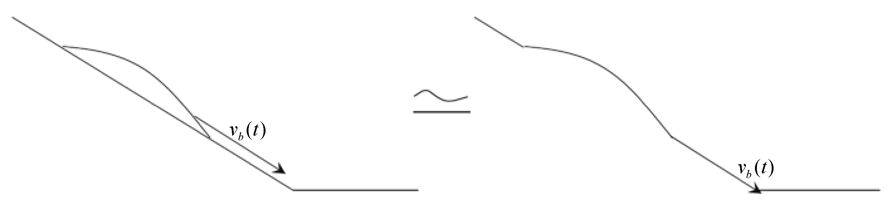
A meshless method is used here to deal with the moving boundary problem. Because it is treated as a potential flow problem, the condition on the solid boundary is the no flux condition. It was suggested that the whole boundary on the slope, which includes a sliding bulk and a fixed slope, can be treated as an inclined moving plate on which a bulk is stuck [11]. A sketch of this assumption is shown in Figure 1.

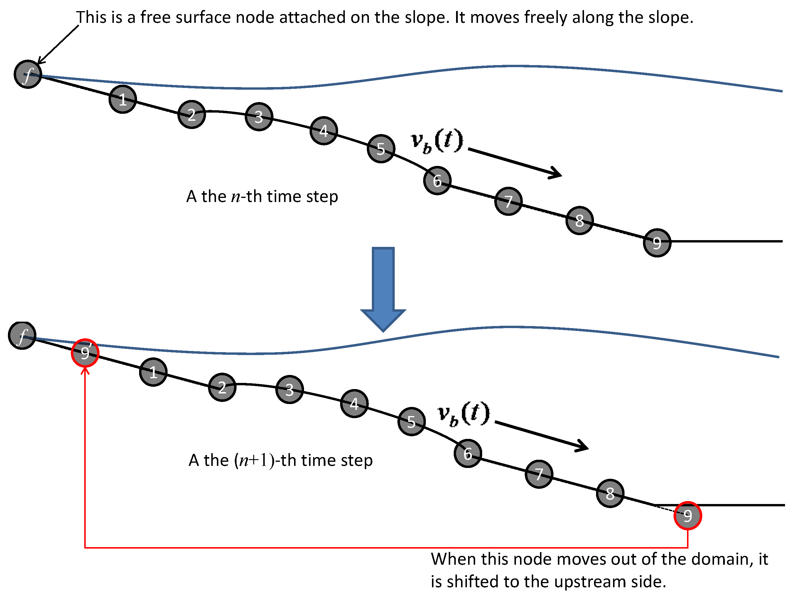
Considering a solid body that moves along the boundary with given velocity ${\overrightarrow{v}}_b(t)$, the collocation points on the moving boundary should move with the velocity ${\overrightarrow{v}}_b(t)$. As the boundary moves, there must be some boundary points going beyond the computational domain at the downstream side. To keep the number of collocation points unchanged in every time step, the out-of-boundary collocation points have to be shifted to the upstream side of the domain with the same interval between points. Figure 2 shows how the collocation points are shifted. It should be kept in mind that the two dimensional plot in Figure 2 is only an illustration sketch. There are thousands of nodes in the three dimensional simulation and the sequence number of the nodes are not just from 1 to 9. In Figure 2 the point $f$ is a free surface node attached on the slope. At this point, two boundary conditions should be satisfied, i.e., $n_{bc}$ equals 2. They are the Dirichlet condition obtained by using Equation (6) and the Neumann condition obtained by using Equation (5). At each time step, the velocity potential $\varphi$ and its spatial derivatives are calculated. Then the position of this point in the next time step can be precisely predicted. Therefore, the movement of the shoreline can be computed.

5. Model Validation

5.1. The Description of the Case

The experiment of the submerged landslide tsunami generation carried out by Enet and Grilli [6] is chosen for the model validation. In the experiment, a rigid body in a streamline shape was placed on a slope initially. The shape of this rigid body is very similar to real landslide bulks. In each run, the rigid body was released suddenly and slid downward along the slope. As it slid, the tsunami was generated. Wave gages were positioned in the water tank to observe the variation of the surface elevation. In this study, we not only compared our numerical results with the experimental data, but also with the numerical results in Fuhrman and Madsen [10]. The water tank in the experiment is 15 m in length, 3.7 m in width. The still water depth is 1.5 m while the slope is 15°. The shape of the landslide model is defined as

$$\zeta =\frac{T}{1-\epsilon }[\mathrm{sech}(k_b\xi )\mathrm{sech}(k_w\eta )-\epsilon ]$$

(33)

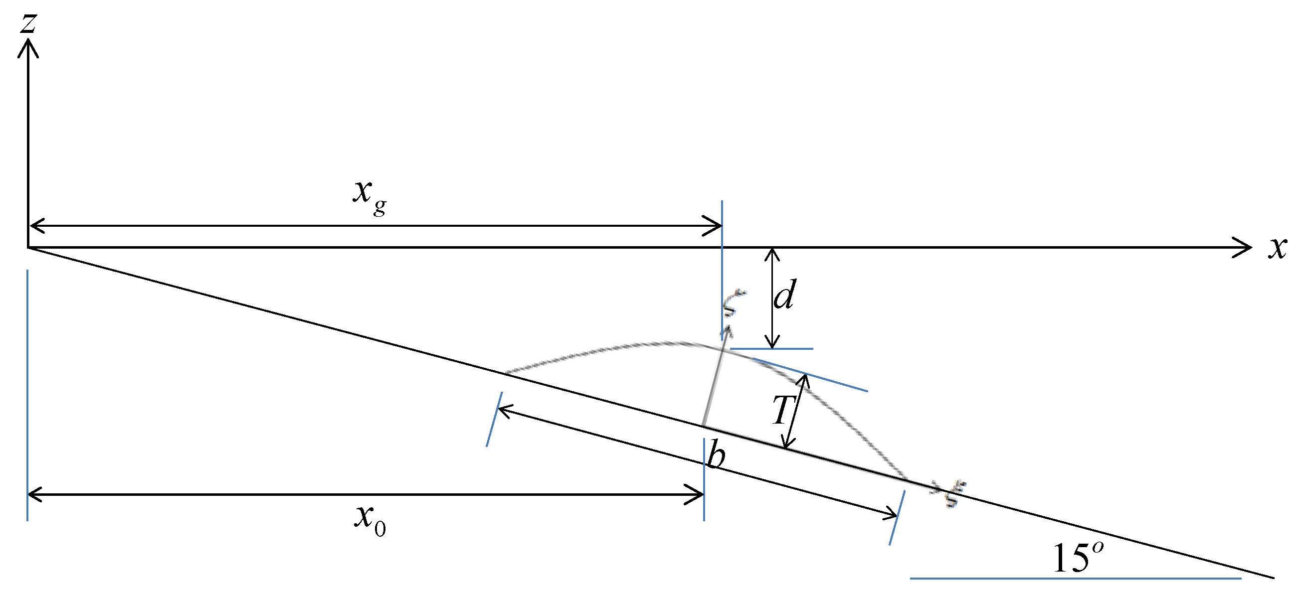
in which $T=0.082\mathrm{m}$ is the thickness, $\epsilon =0.717$ here is a shape parameter, $\zeta (\xi ,\eta )$ is the surface elevation of the landslide model when it is placed horizontally and $\xi$ and $\eta$ are the relative coordinates with respect to the center of the landslide model. The values of $k_b$ and $k_w$ are given by the length and width of the rigid body. They are $k_b=2C/b$ and $k_w=2C/w$ in which $b=0.395\mathrm{m}$ is the width and $w=0.680\mathrm{m}$ is the length, while $C={\cos \mathrm{h}}^{-1}(1/\epsilon )$. Figure 3 shows the geometry of the landslide model and Figure 4 shows the layout of the experiment. Initially, the roof of the landslide model is at $x=x_g$ and the center of the roof of the landslide model is at $x=x_0$ According to Grilli et al. [3], the speed of the sliding body is defined as

$$V(t)=u_t\tanh \left(\frac{t}{t_0}\right)$$

(34)

in which $u_t$ is the terminal velocity of the sliding body and $t_0=u_t/a_0$ is the characteristic time while $a_0$ is the initial acceleration. Three cases for the model validation are listed in

Table 1. Parameters for the 3-D submerged landslide simulations given in Enet and Grilli [6].

Case	$\mathit{d}\left(\mathbf{mm}\right)$	${\mathit{x}}_{\mathbf{g}}\left(\mathbf{mm}\right)$	${\mathit{a}}_0{(\mathbf{m}/\mathbf{s}}^2)$	${\mathit{u}}_{\mathbf{t}}(\mathbf{m}/\mathbf{s})$
1	61	551	1.12	1.70
2	120	763	1.17	2.03
3	189	1017	1.21	1.97

.

5.2. Settings of the Numerical Model

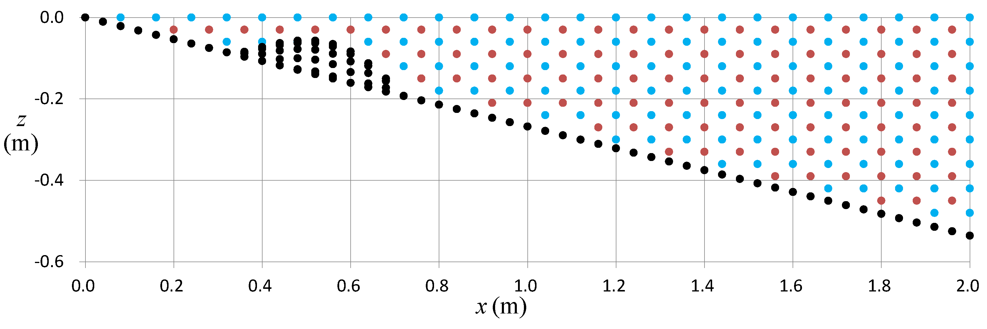
Because the wave flume and the sliding body are symmetric, we choose just half of the channel as the computational domain. The no-flux boundary condition is specified at nodes on the slope, the end wall and the side walls. Dirichlet boundary condition is additional specified at each of these nodes in case it is also on the free surface. Firstly, we distribute the points on the free surface (i.e., $z=0$) regularly, with 8 cm nodal spacing in the x-direction and 8.043 cm nodal spacing in the y-direction. Then, at the plane 3 cm beneath the free surface (i.e., $z=-0.3\mathrm{m}$) we distribute points regularly staggered with the same horizontal nodal spacing. After that we copy the arrangement of the collocation points on the free surface to the $z=-0.6\mathrm{m}$ plane and copy the arrangement of the collocation points on the $z=-0.3\mathrm{m}$ plane to the $z=-0.9\mathrm{m}$ plane, and repeat the same procedure till the computational domain is filled with collocation points. Finally, we remove the nodes that are out of the computational domain and place the collocation nodes on the bottom and the slope, with the 4 cm spacing in the x-direction and 8 cm spacing in the y-direction. The arrangement of initial positions of the collocation points is shown in Figure 5. This is to have the nodes arranged compactly so initially there are enough nodes in the shallow water region above the bulk. The time increment chosen in the computation is 0.01 s.

5.3. The Results

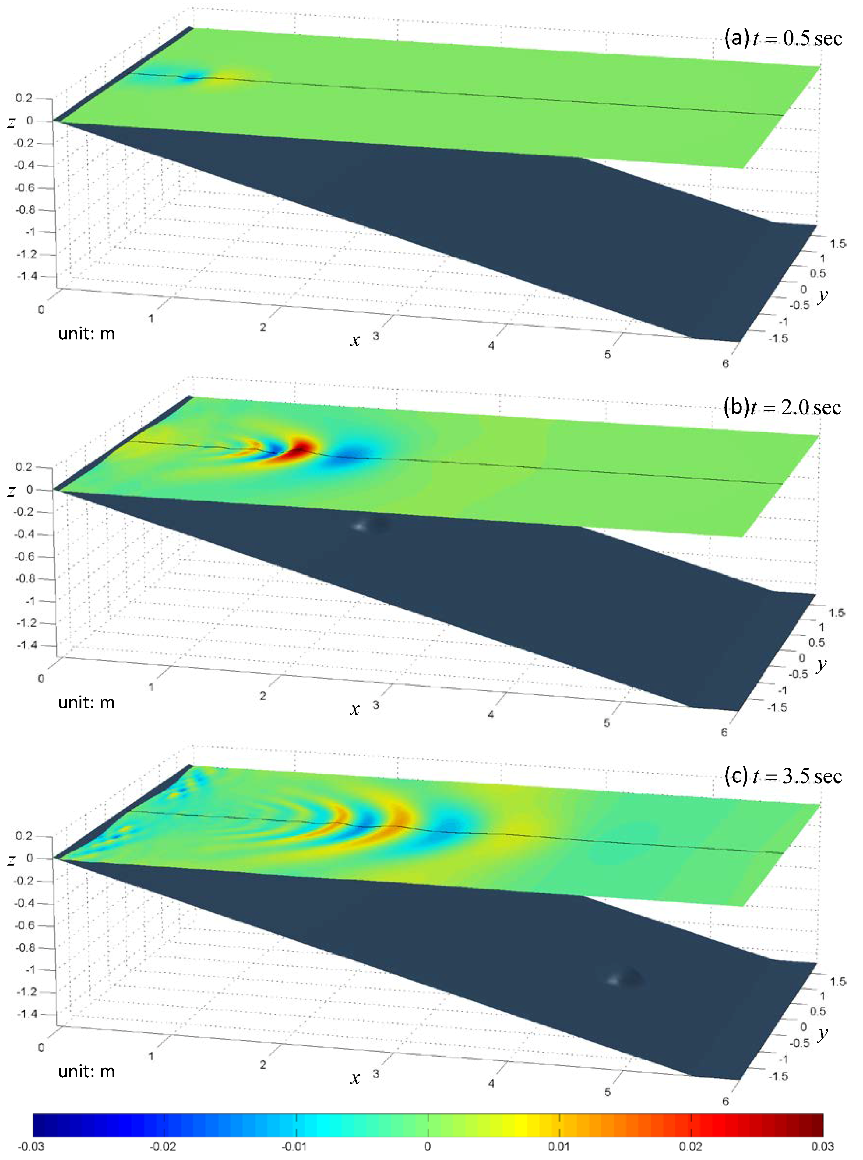
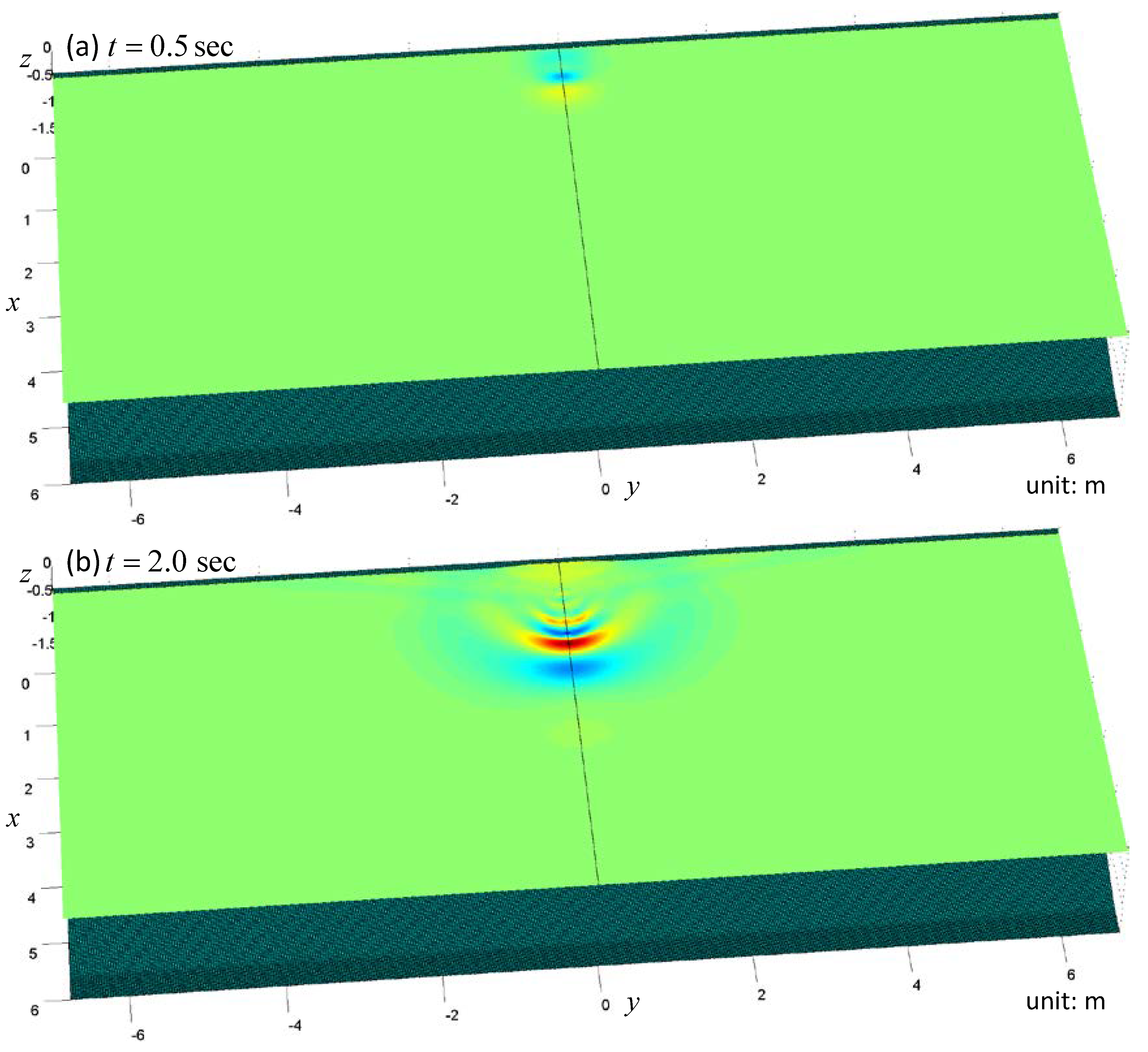
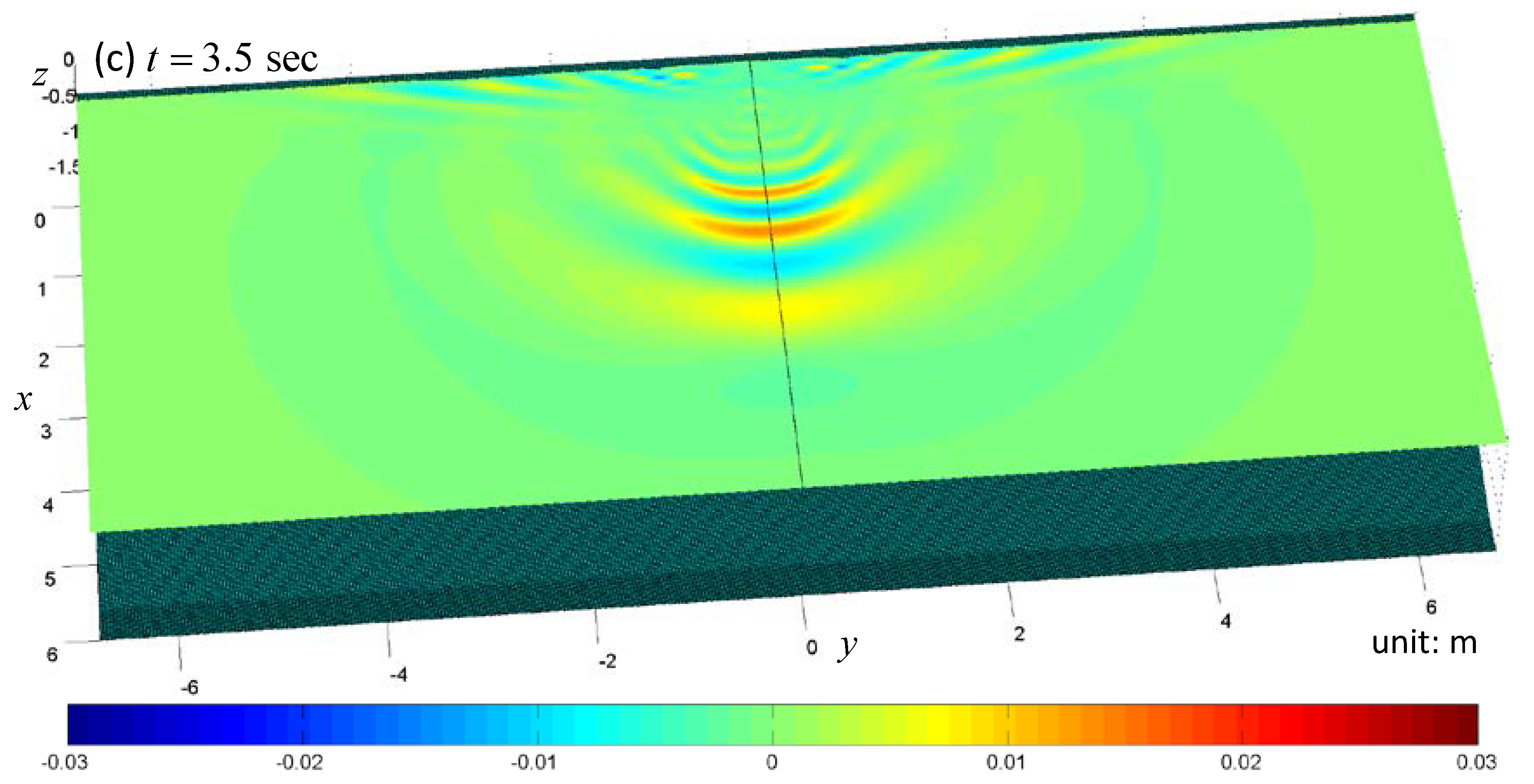
The snapshots of the free surface are shown in Figure 6, Figure 7 and Figure 8. To show the 3-D effect and make the figures clear, we add a central line on the free surface and only plot the region of $x\le 6\mathrm{m}$. In the first panel of each case, one can see there is a hump on the free surface pushed out by the sliding body, and a hollow behind the body. This is known as the N-wave [25]. After the N-wave appears, there are two groups of waves propagating toward opposite directions. The main crest propagates to the deep sea region accompanying some trailing waves while the hollow causes the sea shore to run-down first to the lowest point and then run-up. After that the shoreline moves up and down due to the small waves propagating along the shore. The closer the sliding body initially rests to the shore, the easier this phenomenon is observed. One can also see this in Figure 9 which demonstrates the time series of run-up heights at $y=0$.

We also compare the maximal run-up heights in our simulation with the experimental data in

Table 2. Comparison of simulated maximal run-up heights with experimental data presented in Enet and Grilli [6].

Case	Experiment	Present Model
1	6.2 mm	6.2 mm
2	3.4 mm	3.4 mm
3	2.0 mm	2.2 mm

, which shows that in the first two cases the maximal run-up simulated is identical to the experimental data while the maximal run-up height simulated in the third case is a little larger than the observed.

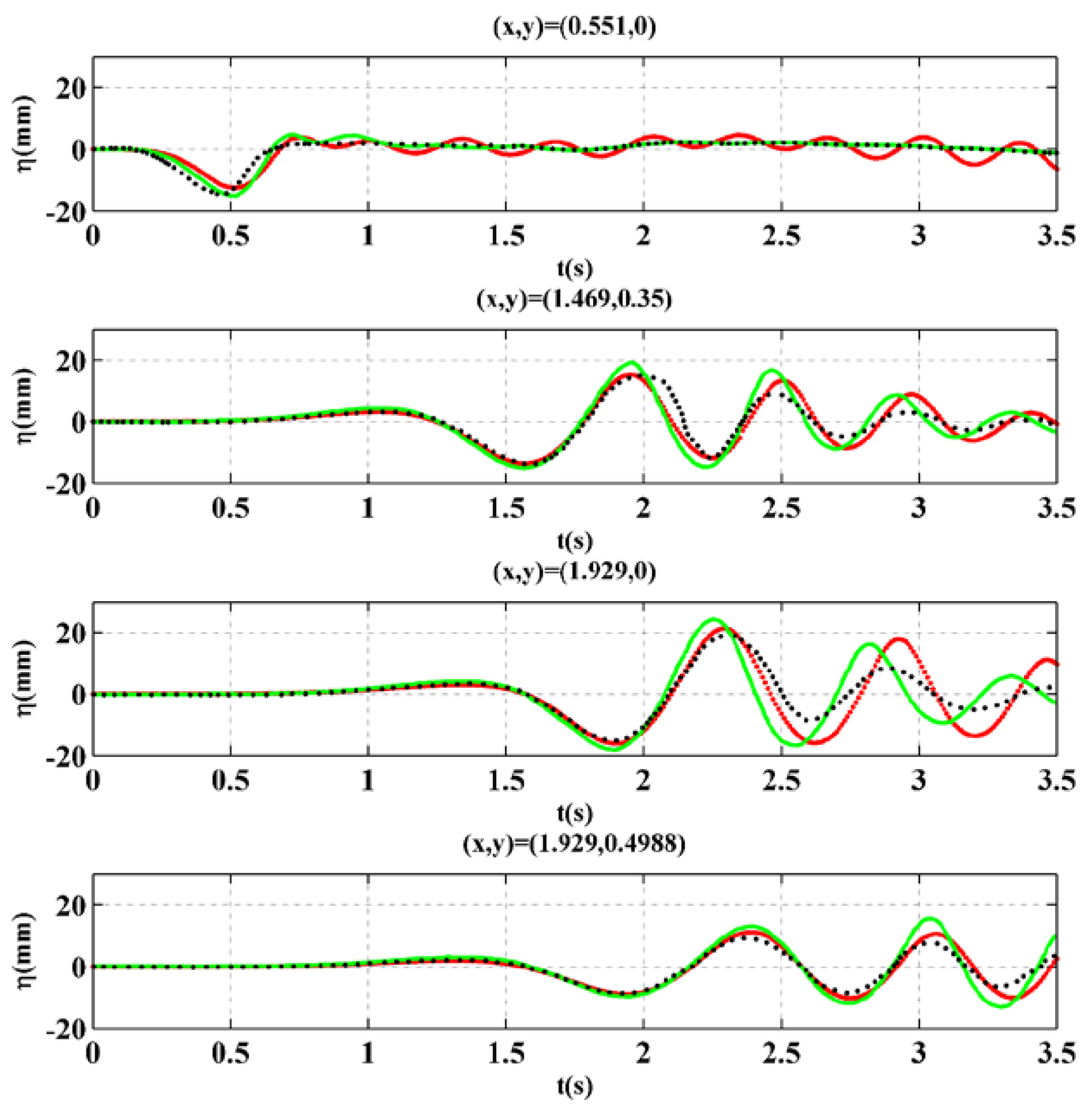
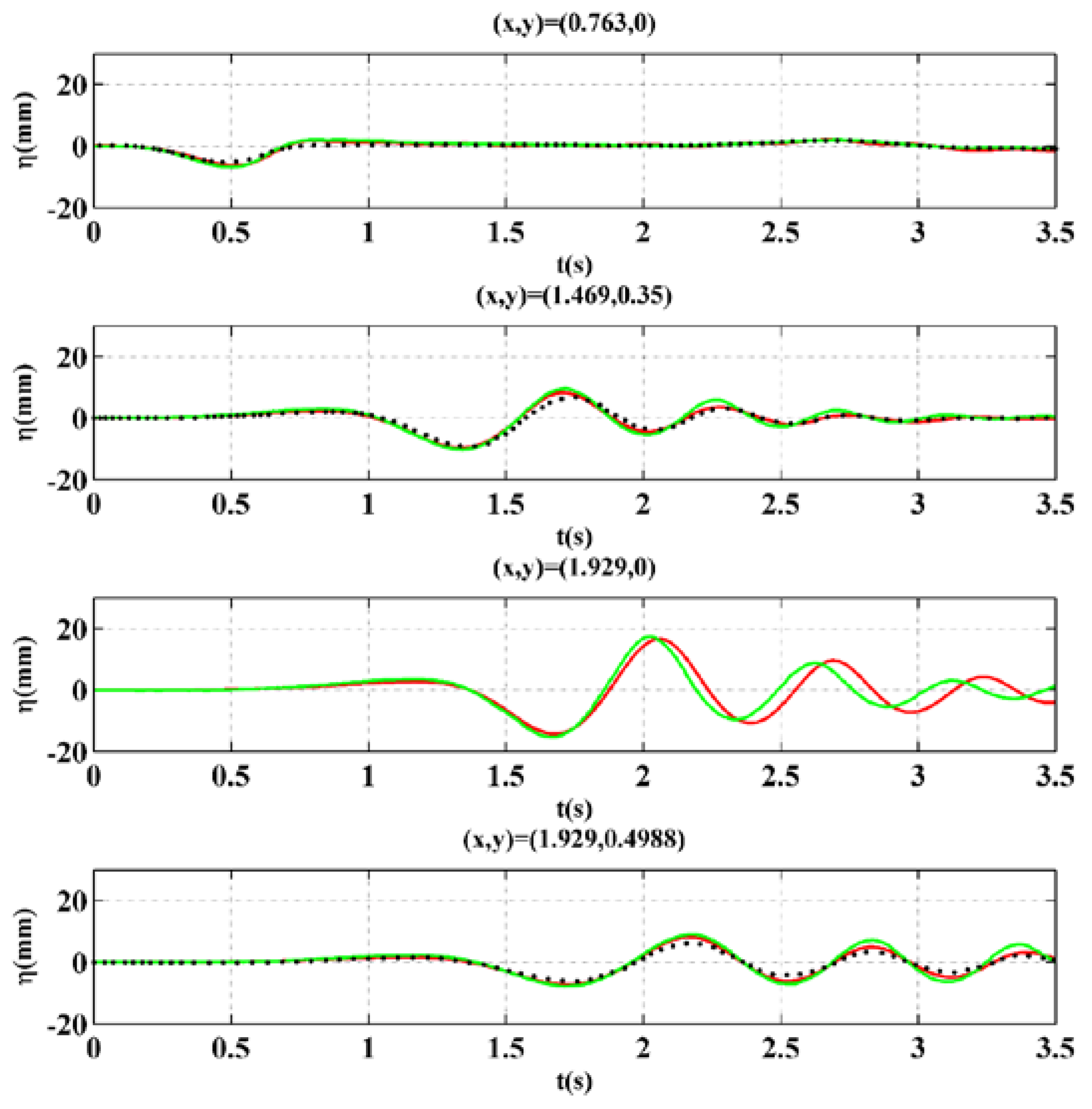
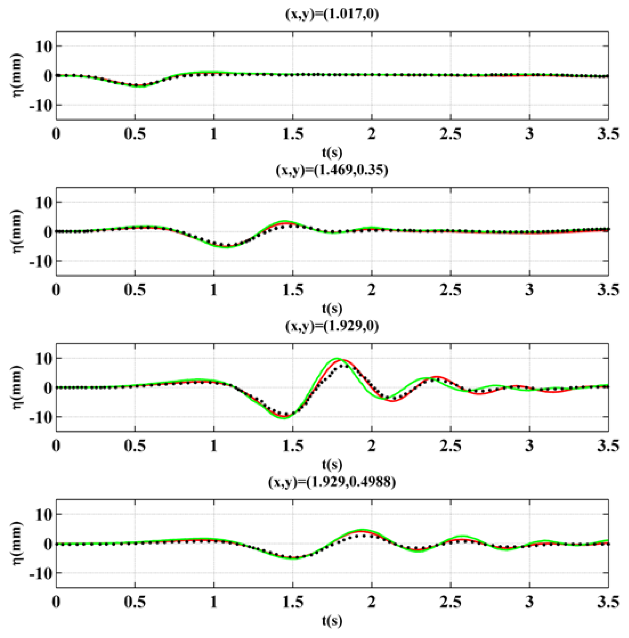
In the experiment, four wave gauges were placed in the wave tank to observe the time series of the free surface elevation. They are at (x, y) = (x_g, 0) m, (x, y) = (1.493, 0.35) m, (x, y) = (1.929, 0) m, and (x, y) = (1.929, 0.4988) m. Because there was missing data at the 3rd gauge in case 2, we could compare our result of this case only with the result in Fuhrman and Madsen [10].

The comparisons of the present results with experimental data and other results are shown in Figure 10, Figure 11 and Figure 12. Besides at gauge 1 in case 1, comparisons show that the present results are very close to the experimental data as well as the results in Fuhrman and Madsen [10]. One can find that even though there are some discrepancies in the comparison, especially at (x, y) = (1.929, 0) m, the present model performs better than the higher-order Boussinesq model [10].

6. Edge Waves

It was mentioned that tsunamis caused by submerged landslides could have a second run-up which might exceed the first one [9]. It is very interesting that the second run-up exceeds the first one at a position other than the position of the landslide. To study this, we simulated the three cases with a 13.52 m wide wave flume, which is 10 times the width of the submerged sliding body and 3.654 times of the flume width in the experiment [6]. In case the sliding body touches the flat bottom, the sliding stops. The simulation is in the time interval of 0–3.9 s.

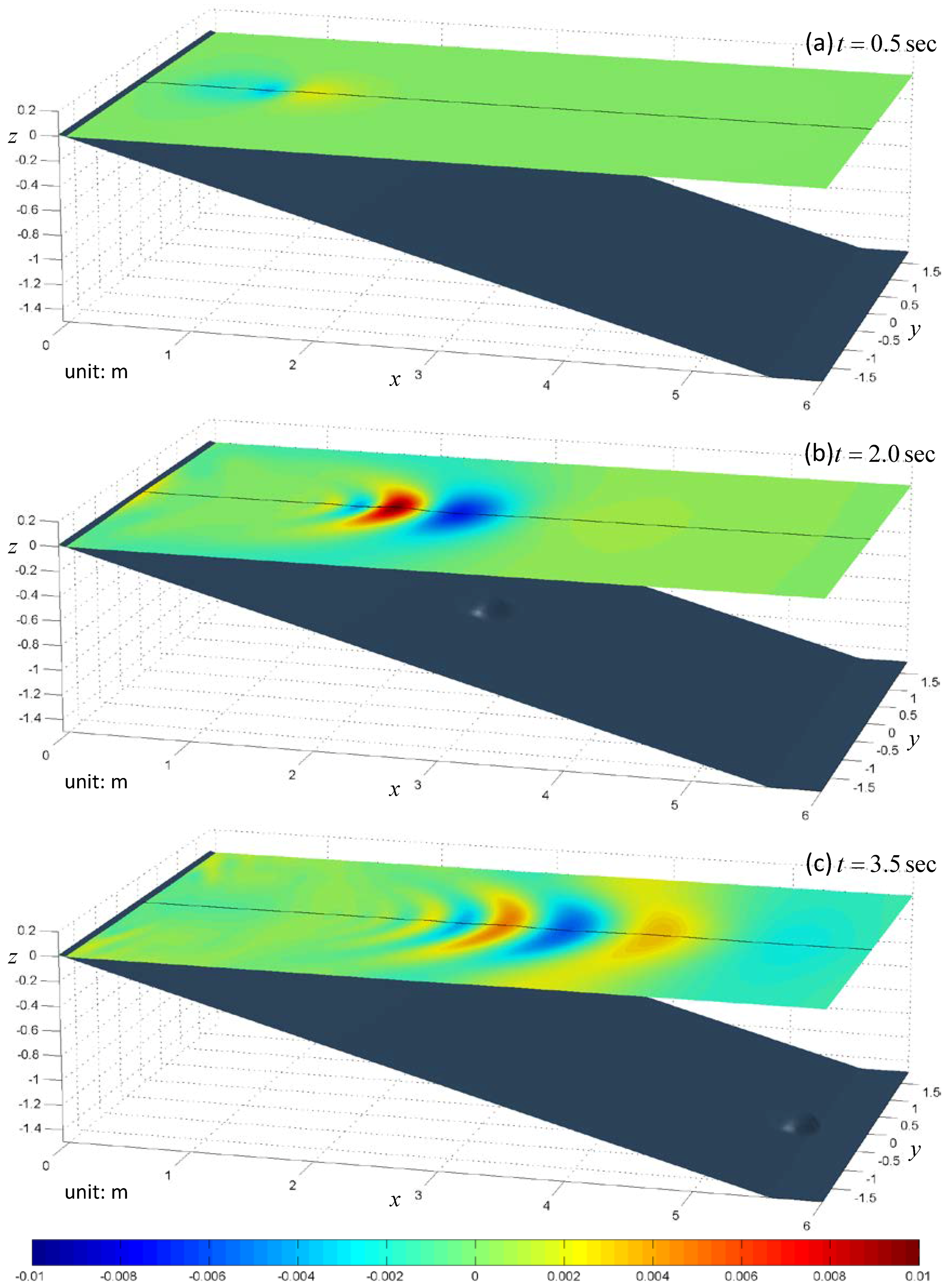
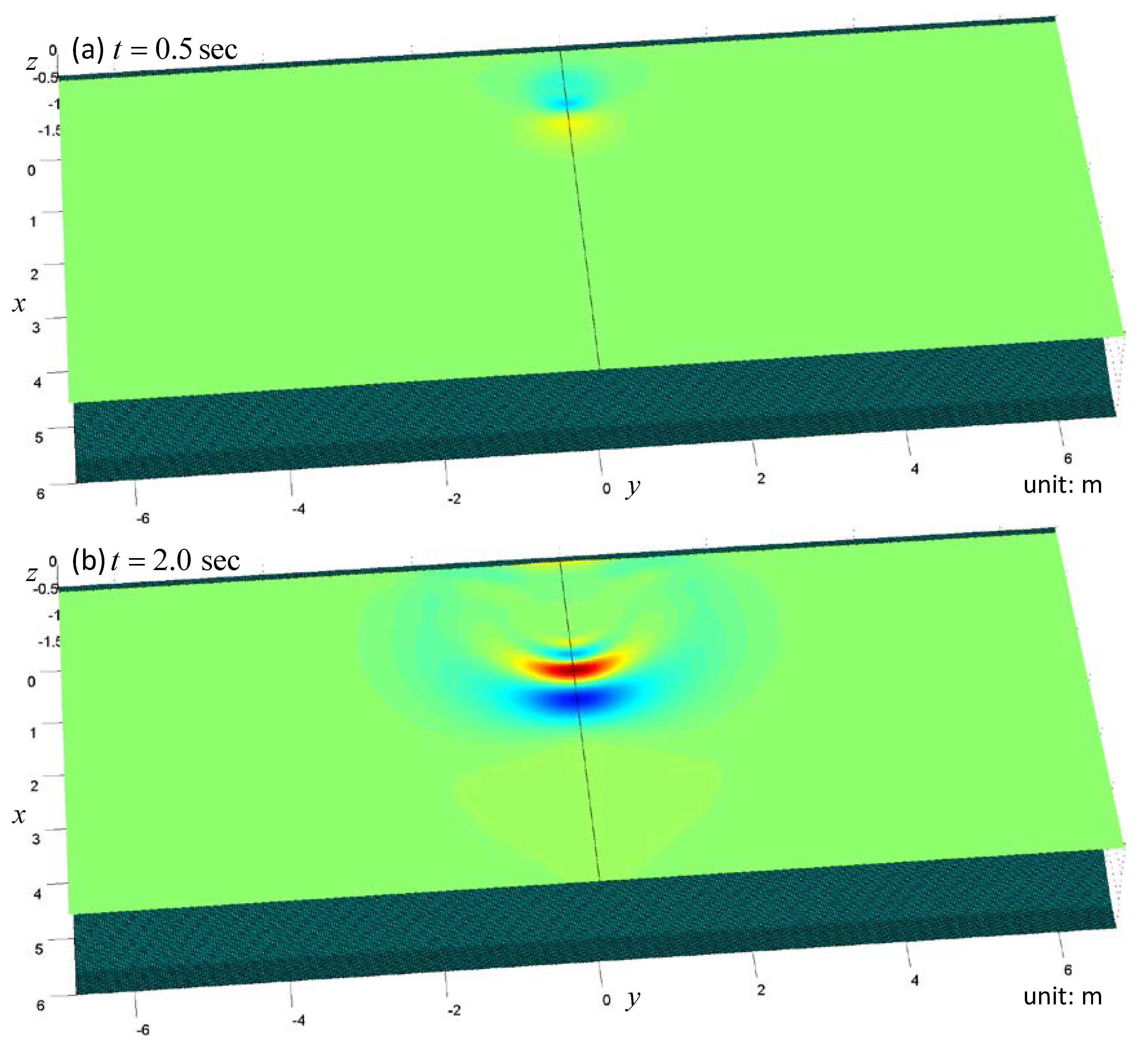
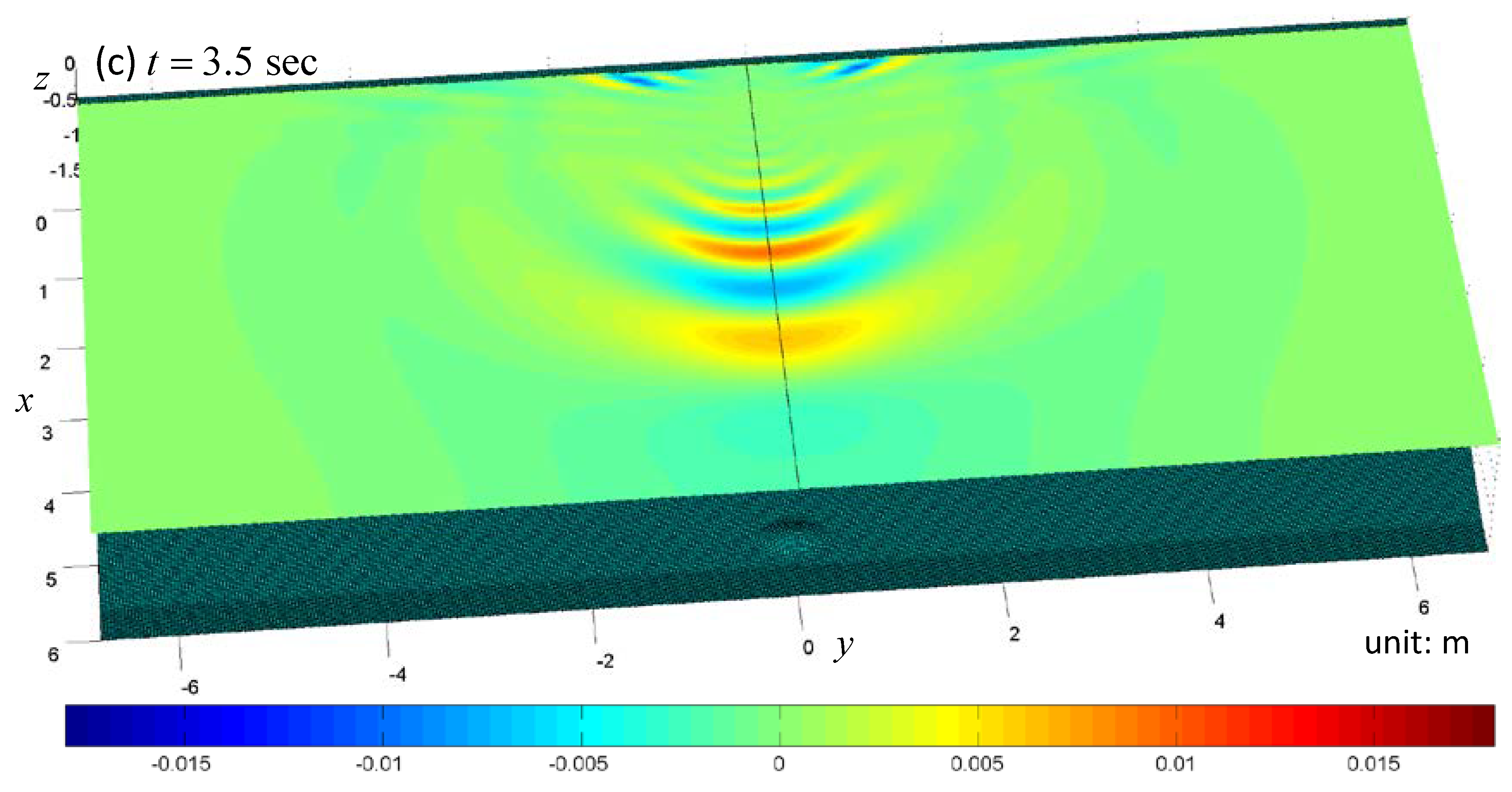
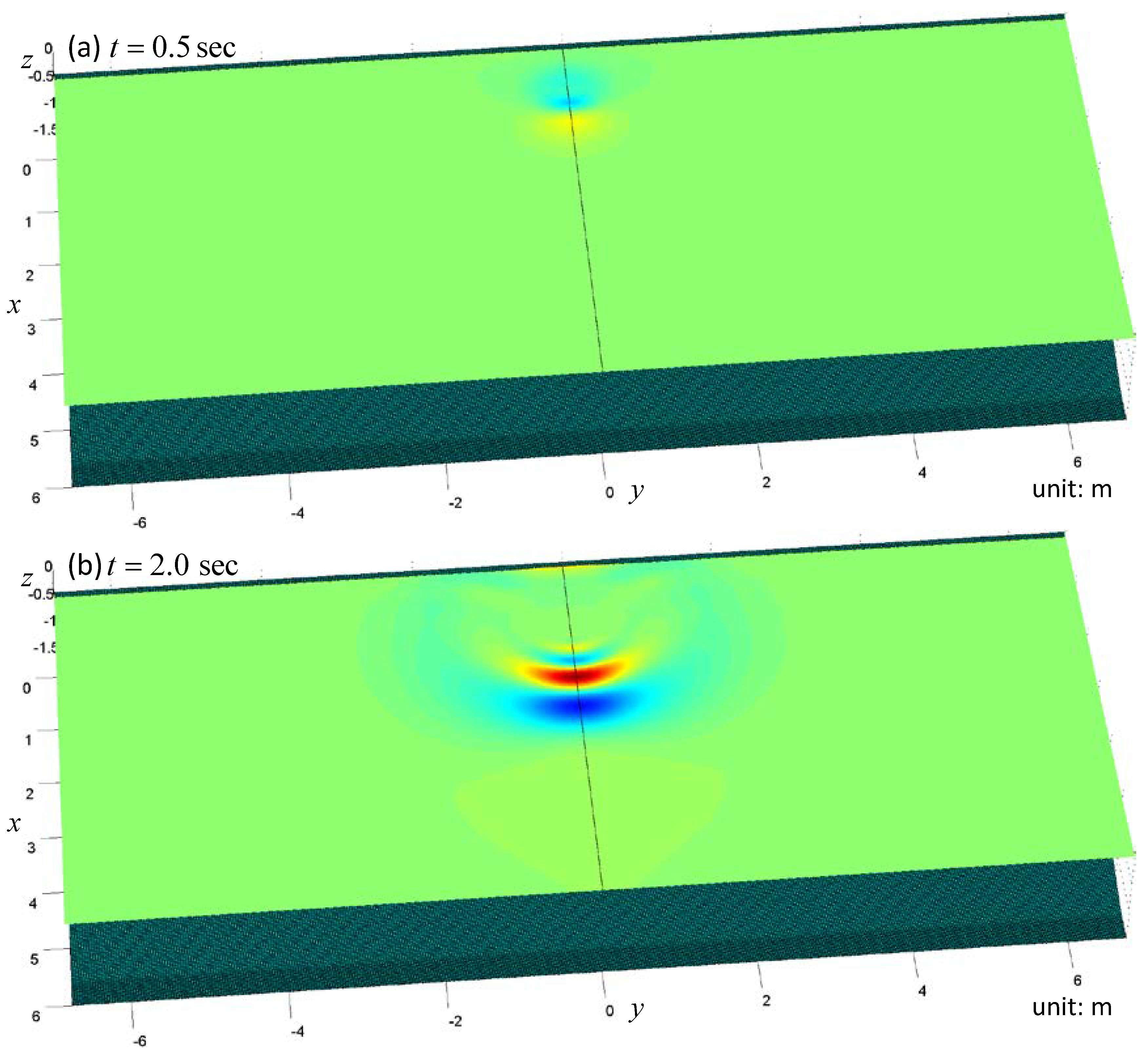
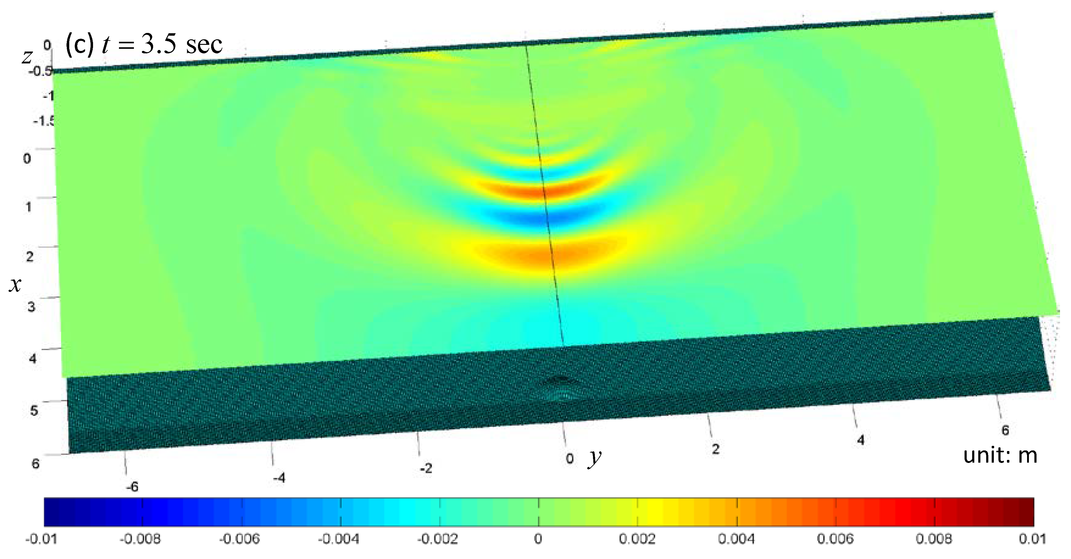
The snapshots of the free surface are shown in Figure 13, Figure 14 and Figure 15. Only the region of $x\le 6\mathrm{m}$ is shown. In the first panel of Figure 13, one can see the N-wave near the shore. In the second panel of this same figure, one can see the water front running up to the shore. In the last panel, two groups of waves can be found. The first group of waves propagates toward the deep region while the other group propagates along the shore. The same trend of wave propagation can also be found in Figure 6. However, since the flume is widened, the edge waves are more perspicuous. The free surface patterns in Figure 14 and Figure 15 are also similar to those in Figure 7 and Figure 8. Because the initial position of the submerged sliding body is not so close to the shore, the edge waves in case 2 and case 3 are not so obvious as in case 1.

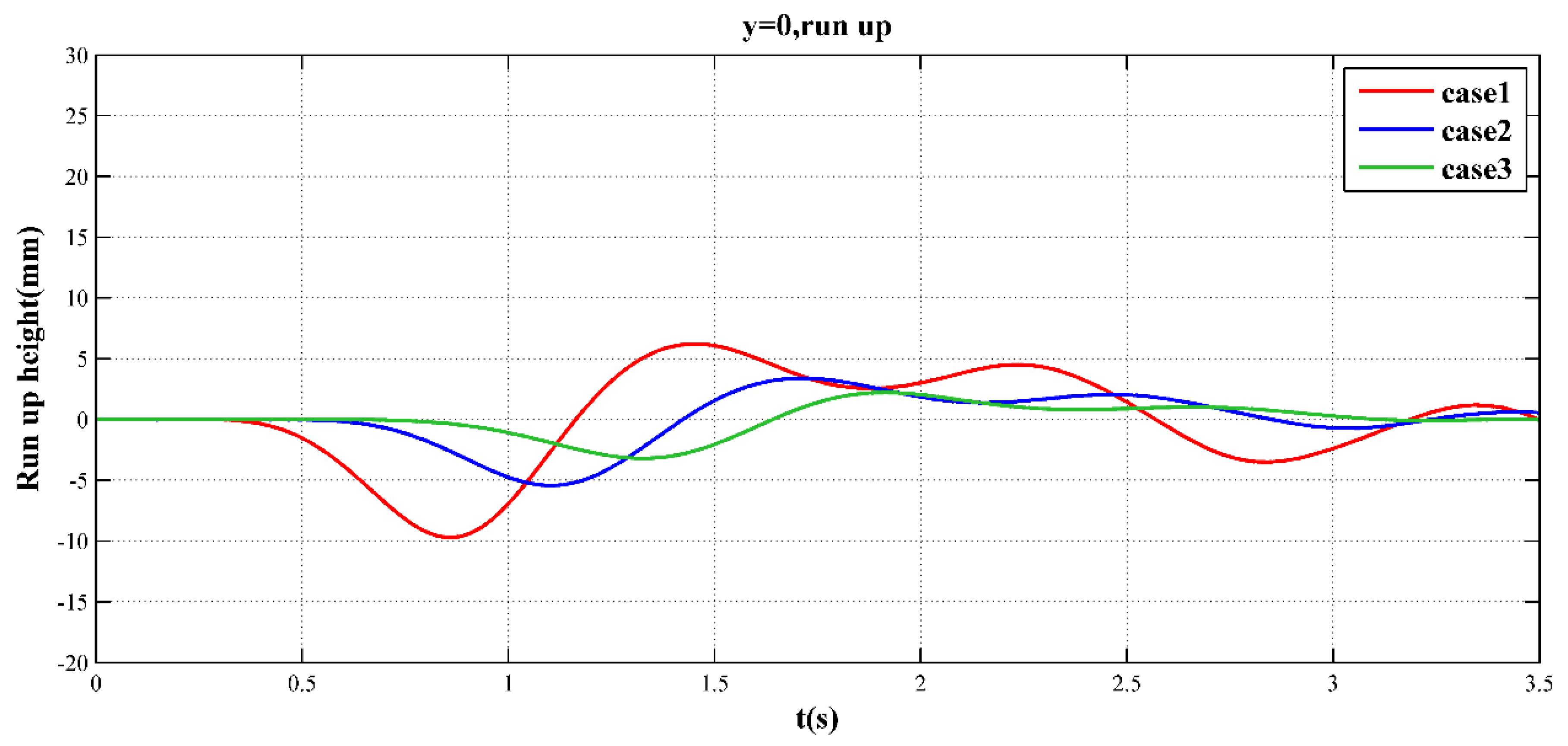
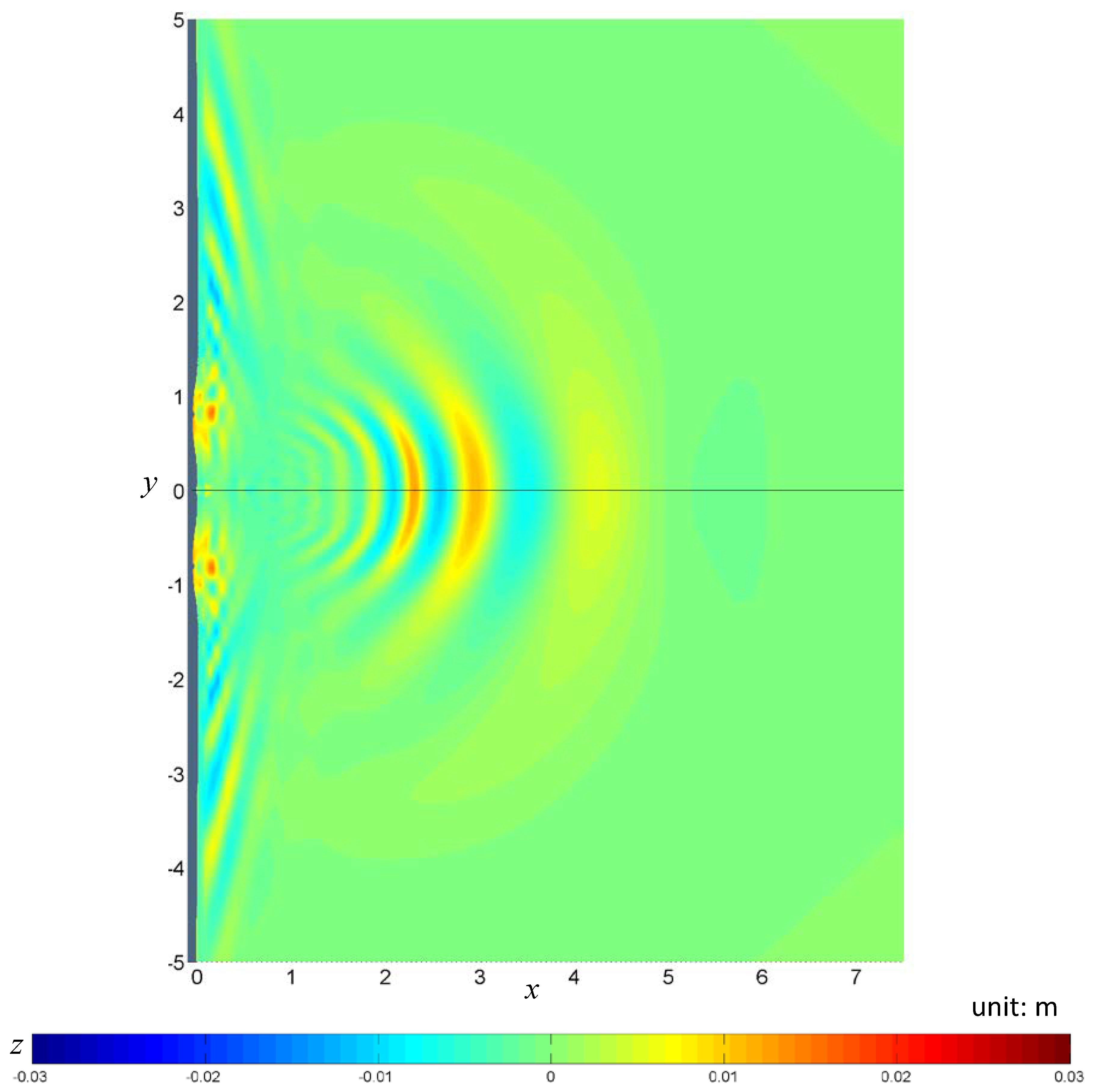
To make a further investigation on the run-up heights, we plotted the time series of the run-up heights along the shore line as shown in Figure 16. In the first panel of this figure, one can see that the run-down comes first at the symmetric point. After that, the land near the shore around $y=0$ is inundated for a while, within which there are two peaks of the run-up. After the flood fades away, the movement of the shore around $y=0$ is relatively calm compared with the other regions. This can also be found in the second and third panels of Figure 13. At t = 3.9 s, a run-up greater than that at y = 0 occurs. The position of this greater run-up is y = ±0.8 m. The patterns of the other two cases are similar. Due to the differences of initial position and velocities, the values are not the same and the greater run-up heights other than at y = 0 do not show up. As the submerged sliding body initially rests closer to the shore, the first run-down comes faster and the first run-up is larger. To see the largest run-up in the simulation, we plotted the distribution of the free surface elevation at t = 3.9 s in case 1, as shown in Figure 17. From this figure and the first panel of Figure 16, one can conclude that the run-up at y = ±0.8 m comes so drastically, after the submerged landslide has occurred for a while.

7. Conclusions

In this study, we developed a numerical model for the simulation of submerged landslide tsunamis. The problem was treated as a potential flow problem so the governing equation is the Laplace equation. The Laplace equation was numerically solved once at each time step by a meshless method. The boundary condition of the sliding bulk on slope was treated as an inclined moving plate on which the bulk is stuck. The present numerical model was validated by comparing the results with experimental data [6] and other numerical results [10]. Good agreement could be found.

After the model was validated, simulations were carried out in a widened wave flume so the edge waves could be further investigated. At the position just behind the submerged landslide, run-down comes first followed by the run-up. The land just behind the submerged landslide becomes flooded for a while and after the flood fades, the movement of the shore is relatively calm compared with other regions. Two groups of waves can be found. The first group of waves propagates toward the deep region and the other group propagates along the shore. In the case that the submerged sliding body rests nearest to the shore, the greatest run-up does not show up just behind the landslide. It shows up at the region other than the place where the land slide occurs. This coincides with the observation in the literature [9].

References

- Mohammed, F.; Fritz, H.M. Physical modeling of tsunamis generated by three-dimensional deformable granular landslides. J. Geophys. Res. 2012, 117, C11015. [Google Scholar] [CrossRef]
- Grilli, S.T.; Watts, P. Modeling of waves generated by a moving submerged body. Applications to underwater landslides. Eng. Anal. Bound. Elem. 1999, 23, 645–656. [Google Scholar] [CrossRef]
- Grilli, S.T.; Vogelmann, S.; Watts, P. Development of a 3D numerical wave tank for modeling tsunami generation by underwater landslides. Eng. Anal. Bound. Elem. 2002, 26, 301–313. [Google Scholar] [CrossRef]
- Grilli, S.T.; Watts, P. Tsunami generation by submarine mass failure. I: Modeling, experimental validation, and sensitivity analysis. J. Waterw. Port Coast. Ocean Eng. 2005, 131, 283–297. [Google Scholar] [CrossRef]
- Enet, F.; Grilli, S.T.; Watts, P. Laboratory experiments for tsunamis generated underwater landslides: Comparison with numerical modelling. In Proceedings of the Thirteen International Offshore and Polar Engineering Conference, Honolulu, HI, USA, 25–30 May 2003; pp. 372–379. [Google Scholar]
- Enet, F.; Grilli, S.T. Experimental study of tsunami generation by three dimensional rigid underwater landslides. J. Waterw. Port Coast. Ocean Eng.-ASCE 2007, 133, 442–454. [Google Scholar] [CrossRef]
- Lynett, P.; Liu, P.L.-F. A numerical study of submarine-landslide-generated waves and run-up. Proc. R. Soc. Lond. A 2002, 458, 2885–2910. [Google Scholar] [CrossRef]
- Lynett, P.; Liu, P.L.-F. A two-layer approach to wave modelling. Proc. R. Soc. Lond. A 2004, 460, 2637–2669. [Google Scholar] [CrossRef]
- Lynett, P.; Liu, P.L.-F. A numerical study of the run-up generated by three-dimensional landslides. J. Geophys. Res. 2005, 110, C03006. [Google Scholar] [CrossRef]
- Fuhrman, D.R.; Madsen, P.A. Tsunami generation, propagation, and run-up with a high-order Boussinesq model. Coast. Eng. 2009, 56, 747–758. [Google Scholar] [CrossRef]
- Huang, T.-Y.; Hsiao, S.-C.; Wu, N.-J. Nonlinear wave propagation and run-up generated by subaerial landslides modeled using meshless method. Comput. Mech. 2014, 53, 203–214. [Google Scholar] [CrossRef]
- Wu, N.-J.; Chang, K.-A. Simulation of free-surface waves in liquid sloshing using a domain-type meshless method. Int. J. Numer. Methods Fluids 2011, 67, 269–288. [Google Scholar] [CrossRef]
- Idelsohn, S.; Storti, M.A.; Oñate, E. Lagrangian formulations to solve free surface incompressible inviscid fluid flows. Comput. Methods Appl. Mech. Eng. 2001, 191, 583–593. [Google Scholar] [CrossRef]
- Zhou, J.T.; Ma, Q.W. MLPG method based on Rankine source solution for modelling 3D breaking waves. Comput. Model. Eng. Sci. 2010, 56, 179–210. [Google Scholar]
- Koh, C.G.; Luo, M.; Gao, M.; Bai, W. Modelling of liquid sloshing with constrained floating baffle. Comput. Struct. 2013, 122, 270–279. [Google Scholar] [CrossRef]
- Tamai, T.; Koshizuka, S. Least squares moving particle semi-implicit method. Comput. Part. Mech. 2014, 1, 277–305. [Google Scholar] [CrossRef]
- Luo, M.; Koh, C.G.; Gao, M.; Bai, W. A particle method for two-phase flows with large density difference. Int. J. Numer. Methods Eng. 2015, 103, 235–255. [Google Scholar] [CrossRef]
- Luo, M.; Koh, C.G.; Bai, W.; Gao, M. A particle method for two-phase flows with compressible air pocket. Int. J. Numer. Methods Eng. 2016, 108, 695–721. [Google Scholar] [CrossRef]
- Wu, N.-J.; Tsay, T.-K. A robust local polynomial collocation method. Int. J. Numer. Methods Eng. 2013, 93, 355–375. [Google Scholar] [CrossRef]
- Oñate, E.; Idelsohn, S.; Zienkiewicz, O.C.; Taylor, R.L. A finite point method in computational mechanics. Applications to convective transport and fluid flow. Int. J. Numer. Methods Eng. 1996, 39, 3839–3866. [Google Scholar] [CrossRef]
- Oñate, E.; Idelsohn, S.; Zienkiewicz, O.C.; Taylor, R.L.; Sacco, C. A stabilized finite point method for analysis of fluid mechanics problems. Comput. Methods Appl. Mech. Eng. 1996, 139, 315–346. [Google Scholar] [CrossRef]
- Wu, N.-J.; Tsay, T.-K.; Chen, Y.-Y.; Tsu, I.-C. Simulation of 2D free-surface potential flows using a robust local polynomial collocation method. In Proceedings of the 5th Asia Pacific Congress on Computational Mechanics & 4th International Symposium on Computational Mechanics, Singapore, 11–14 December 2013. [Google Scholar]
- Wu, N.-J.; Tsay, T.-K.; Chen, Y.-Y. Generation of stable solitary waves by a piston-type wave maker. Wave Motion 2014, 51, 240–255. [Google Scholar] [CrossRef]
- Wu, N.-J.; Hsiao, S.-C.; Wu, H.-L. Mesh-free simulation of liquid sloshing subjected to harmonic excitations. Eng. Anal. Bound. Elem. 2016, 64, 90–100. [Google Scholar] [CrossRef]
- Tadepalli, S.; Synolakis, C.S. The run-up of N-waves on sloping beaches. Proc. Roy. Soc. A 1994, 445, 99–112. [Google Scholar] [CrossRef]