The Impact of Shrubby Floodplain Vegetation Growth on the Discharge Capacity of River Valleys
by

Natalia Walczak
1,*, 
Zbigniew Walczak
2,
Tomasz Kałuża
1,
Mateusz Hämmerling
1 and
Piotr Stachowski
3 1
Department of Hydraulic and Sanitary Engineering, Poznan University of Life Sciences, 60-637 Poznań, Poland
2
Institute of Construction and Geoengineering, Poznan University of Life Sciences, 60-637 Poznań, Poland
3
Institute of Land Improvement, Environmental Development and Geodesy, Poznan University of Life Sciences, 60-637 Poznań, Poland
*
Author to whom correspondence should be addressed.
Water 2018, 10(5), 556; https://doi.org/10.3390/w10050556
Submission received: 2 February 2018
/
Revised: 21 April 2018
/
Accepted: 23 April 2018
/
Published: 25 April 2018
(This article belongs to the Section Water Quality and Contamination)
Abstract
:Willow bush growing in floodplains is a dominant form of vegetation in lowland river valleys due to the availability of water and light. Uncontrolled growth of this plant results in a lower capacity of floodplain areas. Vegetation can narrow the active width of water flow, as well as change water flow velocities at hydrometric verticals falling within the floodplain and the main channel. This paper analyses the impact of long-term growth of willow shrubs on flow resistance coefficient values. Both an increase in the average diameter and the density characterised by the average distance between branches have a significant impact on reducing the flow. The adopted research variants were based on data on the growth rate of the most popular species and forms of willow found in the floodplains of the Warta River above the Jeziorsko reservoir. Two research scenarios were analysed, including data from 12 years, on the development of floodplain vegetation. The first scenario included only the change in diameter (vegetation grew on a cultivation plot), whereas the density remained constant. The second scenario investigated the inverse model—vegetation growing in an uncontrolled manner. The analysis of the tests proved the impact of various bush development scenarios on flow conditions. The results, referred to in the available research papers, indicated the importance of the dynamics of shrub development to the local flow conditions. It was stated that reduction in the flow, depending on the analysed scenario, could reach 45% for scenarios in which the only considered factor was the increase in diameter (at a constant density), and up to 70% in the case of increase in the density of vegetation. Thorough knowledge of this phenomenon may help manage and maintain natural river valleys.
1. Introduction
Riverbeds of large lowland rivers are characterised by a great diversity of flow conditions, and their cross-sections predominantly consist of a main channel and relatively extensive floodplains. They are a complex structure in which hydrological processes can affect vegetation and vegetation can affect the processes occurring in the river [1,2,3,4].
Schiechtl and Stern [5] divided this vegetation into three groups clearly differentiated from each other by height and shape:
Scrub (i.e., eared willow, grey willow) is characterized by a small height and a semi-circular or elliptical outline of the cross-section. Thick branches and leaves, as well as an insignificant height, cause increased sedimentation processes during the flow of water in floodplains, filtering floating particles.
Bushes (i.e., black willow, common osier) are characterised by a multi-stemmed shrub and dense leafage along the whole length of plants. The cross-section of bushes is elliptical or rectangular. The presence of leaves enhances sedimentation during the flow of water, whereas branches bending under the water pressure “catch” plants and other impurities flowing in it. This leads to an increase in resistance of the plants being flown and further to intensification of sediment accumulation processes.
Trees (i.e., goat willow, white willow)—this form of vegetation has a main trunk and foliage begins at a certain height. Therefore, it does not significantly affect the conditions of high water flow. Hydraulic resistance of the trees being flown is low.
In the clusters of lowland river vegetation growing in floodplains, willow bushes dominate.
Vegetation located by riverbanks plays an important role in determining water flow conditions. It can be assumed that vegetation defines the flow conditions in the channel during periods of high discharge. Flow conditions at various plant configurations were also investigated among others by [6,7,8,9,10]. Yang et al. [11] studied the hydraulic characteristics of overland flow. The results show that overland flow velocity remains constant at about 10% for vegetation stems. Also, the relationship between the hydraulic resistance and the Reynolds number is negative when no vegetation exists, but positive on a vegetated slope. Many studies have shown that the basic physical properties of vegetation affect changes in resistance, stream velocity, turbulence structure, and even the transport capacity of organic matter [12,13,14,15]. Essential here are the basic parameters of this vegetation: stiffness of branches, their diameter, height, concentration, and the extent to which plants block the cross-section [13,16,17,18]. Location of plants within the cross-section is also a crucial determinant [19]. This is of vital importance both from the point of view of hydraulic engineering and environmental protection [20,21,22,23]. Ishikawa et al. [24] indicate that the friction factor of the channel bed f had a high positive correlation with the density of vegetation. In studies [25,26], it was emphasised that the evaluation of parameters of water flow resistance caused by vegetation is necessary for modelling the water flow, i.e., in river channels or floodplains. Dense clusters of shrubs (dense branch structure, plus a large share of leaves), with additionally deposited plant debris, generate an increase in flow resistance. Shrubs increase flow resistances and cause flood water levels to rise, which in turn may lead to the breakage of flood banks. Many rivers have submerged aquatic vegetation that significantly affects the water flow characteristics in the channel [20,27]. Grunell et al. [1] noticed, on the basis of field studies, that aquatic plants create and modify river systems through, i.e., catching bottom sediments using their roots. As a result, new plants develop quickly (colonize) and diversify the terrain forms such as: river banks, islands, and flood terraces. The influence of riparian vegetations on overall river patterns varied systematically with the spatial density of plants [28] and the effect increased with the densities. Politti et.al. [29] presented the impact of Salicaceae vegetation on fluvial processes and hydrogeomorphic process feedbacks to vegetation. They have proposed a framework that can be used to define habitat requirements and to describe changes in these drivers that might affect the vegetation, with consequences for river morphodynamics. A primary goal in riparian ecology is to develop general frameworks for prediction of the vegetation response to changing environmental conditions [30]. That framework can offer the possibility to transfer information from rivers where flow standards have been developed to maintain desirable vegetation attributes, to rivers with little or no existing information.
The ecological significance of floodplain vegetation is also important and it has been the subject of many studies. Ensuring that there is a balance between river environments and human needs of rivers remains one of the most important topics of our time [31].
Deciduous species growing on floodplains and river banks include, for instance, poplars (Populus spp.) and willows (Salix spp.). Due to their specificity, these areas cannot be used for typical agricultural production because temporary flooding might destroy crops. The establishment of energy willow plantations may become an alternative. Willow (Salix viminalis L.) is one of the main and most common species in moist places on rivers and streams. It requires a huge amount of water during its growth, and seems to grow well on different soil types apart from the most condensed clay soils and the most coarse-grained sand soils. The soil must not, however, be too acidic or alkaline. It is resistant to adverse climatic conditions and is characterised by high dynamics of growth in subsequent growing seasons and also high biomass production potential. Batz et al. [32] observed that hydrological factors (availability of groundwater and precipitation variability) significantly contributed to the growth rate of willow. Where the groundwater was at a high level, the development of shrub vegetation was noticeably faster and it was responsible for decreasing the active part of the main channel. Consequently, it can be successfully cultivated for energy purposes and might be treated as a long-term source of renewable energy. The profitability of willow energy plants essentially depends on the establishment costs of the plantation, harvesting costs, and anticipated production period of the plantation.
The advantage of using energy willow for cultivation in floodplain areas is that it does not degrade the environment in the way that monoculture farming does. This approach is all the more desirable because shrubby vegetation (willow, wicker) is an element that naturally and often expansively inhabits floodplains and riparian areas.
Research on the development of the energy willow production system has continued in Sweden for over 30 years [33]. Haughton, et al. [34] predicted that over the next 20 years in the UK, bioenergy crops could occupy significant rural areas. The UK government’s Biomass Strategy suggests that bioenergy crops could occupy some 1.1 million ha by 2020. Lisowski [35] made an assertion that the experiences of countries, i.e., Australia, Brazil, Denmark, Finland, Ireland, Canada, Germany, Norway, Sweden, the United States, the United Kingdom, and Italy relating to energy willow cultivation are diverse, and recommendations regarding the methods of harvesting energy vegetation crops are the result of numerous factors that should also be included in Polish climatic conditions. Gullberg [33] observed that the energy willow used in the area of their study only showed an upward trend in the first three years. The regularity was confirmed by [36], who stated that the most intense growth of wood biomass occurs in the third year after founding the plantation. In Sweden and the UK, shrub willow yields are similar to those in Poland, with a value of 8–12 t∙ha−1∙year−1 (up to 20 t∙ha−1∙year−1 in favorable conditions and with high mineral fertilization) fresh mass on production plantations [37,38,39]. This means that the production of willow biomass is four to six times greater than the annual growth of wood in forests. According to Scandinavian studies, willow harvest in three to five-year cycles is the most economically justified [40]. Whereas Kopp et al. [41] conducted research on five willows and one poplar species (as an example of energy plants) and they cultivated them for 10 years. Half of the trees were fertilized annually, and all trees were irrigated, starting from the third vegetative season. Annual biomass production ensured that well-adapted willows could be cultivated/exploited for at least 10 years. Fertilization did not increase the achieved level of maximum biomass production, but it shortened the time required for maximum production by one year.
Vegetation of floodplains is also often a refuge for fauna, especially waterfowl. Middle Warta River Valley is an element of the ECONET-PL network as a node area 19M [42], and is listed as a mainstay within the CORINE biotopes network. This area is also a bird mainstay on the European level-PL076 Middle Warta River Valley [43], especially for water birds.
However, it should be remembered that natural vegetation growing in an uncontrolled way can pose additional risk in the event of high water or impoundment. Therefore, the growth of vegetation, especially in floodplains, should be constantly monitored and controlled, in a traditional way or with the use of laser scanning [44].
However, in terms of flood flows, more important is the impact of flood vegetation on the safe conduct of flood waves [45,46]. Conditions for flood wave transformation in the river valley are significantly affected by the actual state of the channel and its floodplains. Flood vegetation may affect the rate of flood wave propagation, in particular for floods with a higher probability of occurrence, where the peak of the flood wave is lower. Rate of flood wave propagation, for the low roughness cases, is also two to three times greater than for the high roughness cases [47]. In addition, riparian vegetation participates in the transport of organic matter [48,49,50] by stopping plant debris in the shrub zone, which may cause a decrease in the capacity of the channel [51]. Vegetation also plays an important role in controlling riverbed erosion [52,53] and sediment processes [48,54,55]. Plant debris may additionally affect economic losses, e.g., on grates in hydroelectric power plants [56].
For the purpose of this work, the impact of long-term growth of willow shrubs on the values of flow resistance coefficient was analysed. The adopted research scenarios were based on data on the growth rate of the most popular species and forms of willow found in the floodplains of the Warta River above the Jeziorsko reservoir.
2. Materials and Methods
2.1. General Characteristics of the Research Area and Field Measurement
According to the available data (GUS—the Central Statistical Office, OTKZ—the Centre of technical inspection of dams), the Jeziorsko reservoir on the Warta river is the second largest storage reservoir in terms of flooding area, and the fourth largest in terms of capacity among 71 large storage reservoirs in Poland (height of the dam above 15 m or capacity over 3 million m3). The intensive growth of shrubby vegetation (willow shrubs) in the upper part of the reservoir and its floodplains within the embankments above it has been observed since regulatory works were completed in 1985. Before the construction of the reservoir, the area of the Warta valley was owned by private farmers and used for agricultural purposes, such as meadows and pastures. Willow bushes grew in the vicinity of oxbow lakes and ponds in the river valley and along the banks of the main channel.
The purchase of land in the reservoir bowl and in the backwater zone made by the State Treasury contributed to the disappearance of agricultural activity in these areas. With the simultaneous lack of maintenance works, the areas were exposed to the intensive growth of willow bushes. Shrubby vegetation does not occur in places where embanked areas are used as pastures. The analysed area of shrubby vegetation growing in an uncontrolled manner (Figure 1) on the flood plains of the Warta River has been studied for many years, including, i.e., the influence of floodplain vegetation on the flow rate, longitudinal and down erosion, and granulometric composition of debris. For their research, the authors selected a typical section of the Warta River. The analysed area concerned the lowland river characterised by wide floodplains. Floods on the Warta river occur both in early spring periods (vegetation without leaves) and in summer periods (foliage vegetation). On the basis of site visions and photographic documentation, it is possible to estimate that approx. 50% of the analysed floodplain area was covered by shrubs in the form of compact complexes, and the rest of the area was comprised of reed and grass. The left-bank side of the analysed area was more overgrown than the right-bank side since the farmers had not used it as pastures and meadows. The area was mainly overgrown by willow, but there were also trees.
A full inventory of vegetation consisting of measuring all shrubs and bushes is not possible. However, the method of shrub inventory that lies in testing not all of the studied area, but only a part of it (i.e., a test area), can be used. The application of the statistical method of plant inventory makes it possible to determine plant parameters for both small and larger areas. This method consists in drawing conclusions with regard to geometrical parameters based on a sample taken in accordance with the principles of mathematical statistics [57]. Statistical inventory consists of measuring an arbitrarily large number of taxonomic features at strictly defined points. It is assumed that the value of each feature measured on a given surface is treated as the value of a random variable. The standard error of the estimate of plant parameters cannot exceed the assumed error tolerance. The number of test areas, in accordance with de Vries [57], was estimated at n = 3. The size of test areas should depend on local conditions in such a way as to measure the optimal number of shrubs and bushes, both from the point of view of the costs of fieldwork and for the accuracy of the results. For willow bushes, where the average number of branches is L = 100 pcs/m2, and the appropriate number of branches that need to be tested should vary from 50 to 100 pieces, the optimal size of the test area is 0.5 to 1 m2.
The field measurements of vegetation were carried out for the first time from 30 August to 3 September 2004. Then, they were continued in subsequent years: 11–16 July 2005 and 5 April 2006, including a section of the river from 503 to 508 km. The height of willow bushes in the reservoir and in the flood areas within the embankments ranged from 3.0 m to 5.0 m. The measurements of bush structure were made using the methodology described in research journals [58]. The local inspection carried out in the analysed areas showed various forms of shrubs. In some places, compact clusters of bushes were observed, and in others, single scattered plants were seen; sometimes, there willow plantations cultivated for regulatory works were found.
For the purpose of the study, the authors selected three areas (a, b, and c) of the floodplains of the Warta River covering the section from 505 + 720 km to 504 + 730 km (Figure 2). They represented forms of willow typical of the Central European lowland rivers. These areas were characterized by vegetation at various stages of development. The method of measuring the spacing and diameter consisted of choosing the model area of 1.0 m2 in each of the selected areas and the exact inventory of all major woody elements of the plants, including the main stems, the branches, and smaller twigs (a, b, and c areas selected as representative of the considered section of the river). The diameters and the spacing of the different woody plant parts were measured using calipers and a measure, respectively. The obtained results were then averaged to obtain a representative mean diameter and distance. It was assumed that the spacing in the direction of flow and transversely to it was equal.
2.2. Methodology
Floodplain vegetation is defined with the use of geometric parameters describing its structure i.e.,: dp—diameter of bush branches, and ax and ay—spacing between bush branches in both directions of flow. The initial values of geometrical parameters (diameter and spacing) of shrub vegetation concerning data from 2004 and 2005 were adopted on the basis of an inventory made during field measurements. The data was used as the input for simulations covering another 11 years of growth.
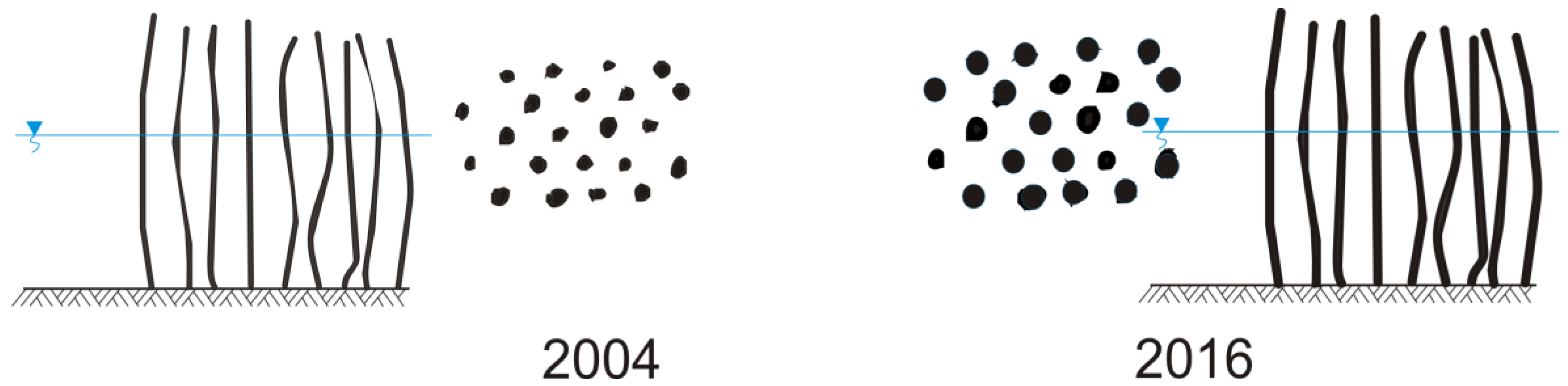
While assessing the capacity of the Warta River valley, the authors thoroughly analysed two scenarios that most often occur in floodplain areas. The first scenario (I) studied the vegetation (Figure 3) on the understanding that it grew on a cultivation plot (willow plantation). Therefore, in accordance with the adopted growth scheme for energy willow [59], the diameter was assumed to increase by a constant 10% over all years of simulation tests. However, the spacing was assumed to remain unchanged, differing by only approx. 2‰. Such values justify the usefulness of growing plants for energy purposes, in this case, energy willow, since thicker shoots are a more valuable fuel material.
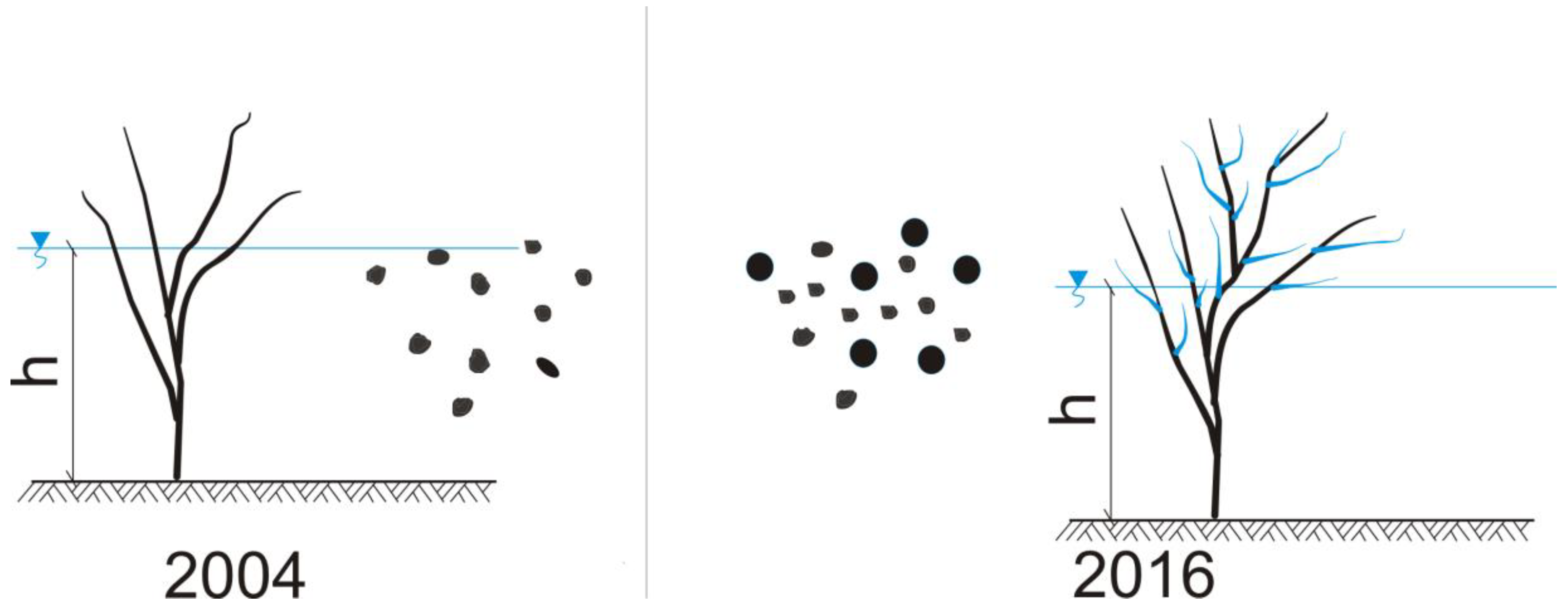
The second scenario (II) considered the vegetation with parameters variable over time, because it increased its lateral surface by developing additional shoots (Figure 4). As a result, the diameter did not change significantly (by 2% during 12 years of simulation), whereas the spacing decreased due to the appearance of younger shoots (yearly by 10%).
The range of variability in diameter values was confirmed by Kałuża’s research in 2009 [58] (Figure 5), which included the three most common trees found in floodplains (pine, oak, poplar). Only the diameter parameter could be used in simulations, and the spacing of this type of vegetation (trees) did not correspond with the typical shrub vegetation analysed in the paper. The increase in the parameters of shrub vegetation in scenario II was modelled on the basis of the forest growth and yield tables, as well as the available literature [58,60,61]. The disadvantage of this extrapolation is the fact that the data contained therein does not apply to bushes, but only to trees. All the manuscripts contain the increase in diameters and spacing following in subsequent years. The authors decided that the vegetation growing under the same soil and climatic conditions would have a similar growth rate. For scenario I, the parameters of energy willow were adopted on the basis of publicly available data for prospective producers [62].
In the overgrown part of the channel, flow resistances depend on both vegetation and roughness of the bottom. The total resistance coefficient in this area is the sum of partial coefficients [63]:
λ = λp + λd
Dimensionless coefficient of flow resistance λp, which is calculated taking into account the share of cross-sectional area occupied by willow branches to the surface of the entire cross-section, can be determined based on the equation:
where:
CWR—resistance coefficient for group of tress
dp—average bushes diameter (m)
ax, ay—distance between willow branches in the direction of flow and transverse to it (m)
h—height of the submerged plant (m)
α—the angle of inclination of the bottom in the direction transverse to the direction of flow
λd—bottom resistance coefficient.
The friction factors for high vegetation were the object of investigations by Lindner [64] and Pasche [65]. Equation (2) was determined for the flow of water around the tree based on experimental studies with cylindrical elements. The experiments were conducted using a vegetation density of 50 elements per m2 produced with PVC cylinders of 10 mm in diameter and 150 mm in height. Equation (2) can be used for both high vegetation and medium-height plants [66,67].
It is convenient to determine the resistance coefficient CWR according to the formula modified by Rickert [68]:
where
dp—diameter of a willow twig (m)
ax, ay—distance between willow branches in the direction of flow and transverse to it (m)
—ratio of water velocity flowing into the bush and the averaged velocity in the cross-section of the channel
h—height of the submerged part of the plant (m)
α—inclination angle of the river bottom in the direction transverse to the direction of flow
CWR—substitute value of the resistance coefficient for a group of plant elements, which depends on the ratio of the velocity and height of waves that arise on the surface when flowing these elements. The CWR = 0.8–1.1 was assumed in the calculations. The first parenthesis takes into account an increase in the resistance coefficient due to the overlapping of disturbances caused by neighbouring plant elements, while the second parenthesis represents the ratio of the water velocity reaching plant elements and the average velocity in the cross-section. The analysed vegetation due to the lack of foliage and post-vegetative season was treated as rigid and non-deformable under the action of water. Therefore, there was no risk of overlapping between plant elements. The authors also decided to use the Rickert’s modification because it directly takes into account the geometrical parameters of shrubby vegetation, i.e., diameter and spacing values (facilitation of field measurements). In addition, the factor takes into account the ratio of the water velocity flowing into vegetation and the average water velocity in the cross-section.
Coefficient of resistance caused by the roughness of the river bottom λd, is calculated using the formula:
where:
R—hydraulic radius, defined as the ratio of the cross-sectional area of stream (A) to the wetted perimeter in this cross-section (U) (m), k—height of bottom roughness (m).
The flow rate value was calculated by the Darcy-Weisbach formula:
where:
R—hydraulic radius, defined as the ratio of the cross-sectional area of stream
I—water slope (-)
It was assumed that the filling of floodplains with water (for scenarios I and II) was 1.0 m high and for this value, the water flow was calculated. Such depth values were achieved during high water in spring 2006 in the flood area of the Warta river above the Jeziorsko reservoir [12]. During the spring flood, the water flow was estimated at: Q = 185 m3∙s−1, the water depth in floodplains reached max. 1.75 m (on average 1.0). The height for bushes ranged from 3.0 m to 5.0 m, and for reed from 0.85 m to 1.0 m, respectively. The velocity measurements were carried out using a 100 mm diameter current meter (Hega II) and they were 0.13–0.26 m/s. The water table slope I = 1.364‰ was determined based on GPS measurements of the water table level in the following cross-sections: 503 + 660 km and 511 + 400 km.
The percentage reduction was determined by analysing the decrease in flow in each year in proportion to the base flow designated in year 0.
3. Results and Discussion
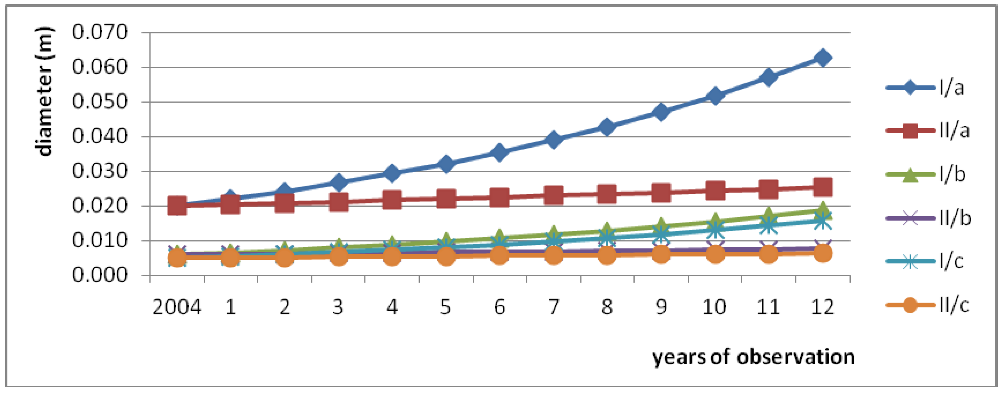
Figure 6 presents the calculated results of change in the diameter for two analysed scenarios (I and II) in three floodplain areas of the Warta River (a, b, c). In the first scenario (I), the diameters significantly changed within 12 years. A long simulation/operation period was applied, i.e., in order to spread the costs of establishing and closing the plantation [69].
In all test zones, the diameters increased threefold. In the second scenario (II), the averaged diameters in zones a and b increased slightly, whereas, the diameter in zone c increased fivefold.
The rate of increase in the diameter of willow cultivated on the plot corresponds well with the data provided in guides for farmers [70] and scientific publications [59,71,72]. In the first year, willow’s diameter ranges from 7 to 13 mm. In the second year, the thickness of the plant increases by 1–2 mm. From the third year on, the diameters increase by 5–10 mm. Depending on the willow species, in the fourth year, the diameter of the shoots reaches 20–40 mm [59].
For the purpose of the graphical representation of data in Figure 7, there were analysed changes of the spacing between branches of floodplain vegetation during 12 years of simulation. In Poland, energy willow (common osier) plantations in most cases (particularly on farms) have a small acreage, and they are substantially distanced from each other [73]. As a result, the rental or purchase of specialised machines is often an insurmountable economic barrier for owners of plantations. Cutting with the use of mechanical saws is a frequent method of willow harvesting [69], and the adopted spacing values are 0.06, 0.1, and 0.12 m, usually being lower than the standard 0.33 m. For vegetation cultivated on natural floodplains, plant protection products are not used, and small spacing makes young shoots grow less intensively.
In scenario II, reduction in the spacing resulted from the natural succession of willow, which despite a stable growth, was subject to changes due to the environmental impact. Analysing the spacing in scenario I within 12 years of simulation, it can be stated that it changed insignificantly, as a result of cultivation maintenance. Cutting out of young shoots is necessary when plantations are run for economic purposes. Additionally, young shoots are used as cuttings, and by rooting, they form new plants [74]. Standard deviations (SD) and coefficient variations (Cv) for the diameters and distance values are included in Table 1. The above values were determined for the entire analysed period, i.e., for 12 years, for individual scenarios.
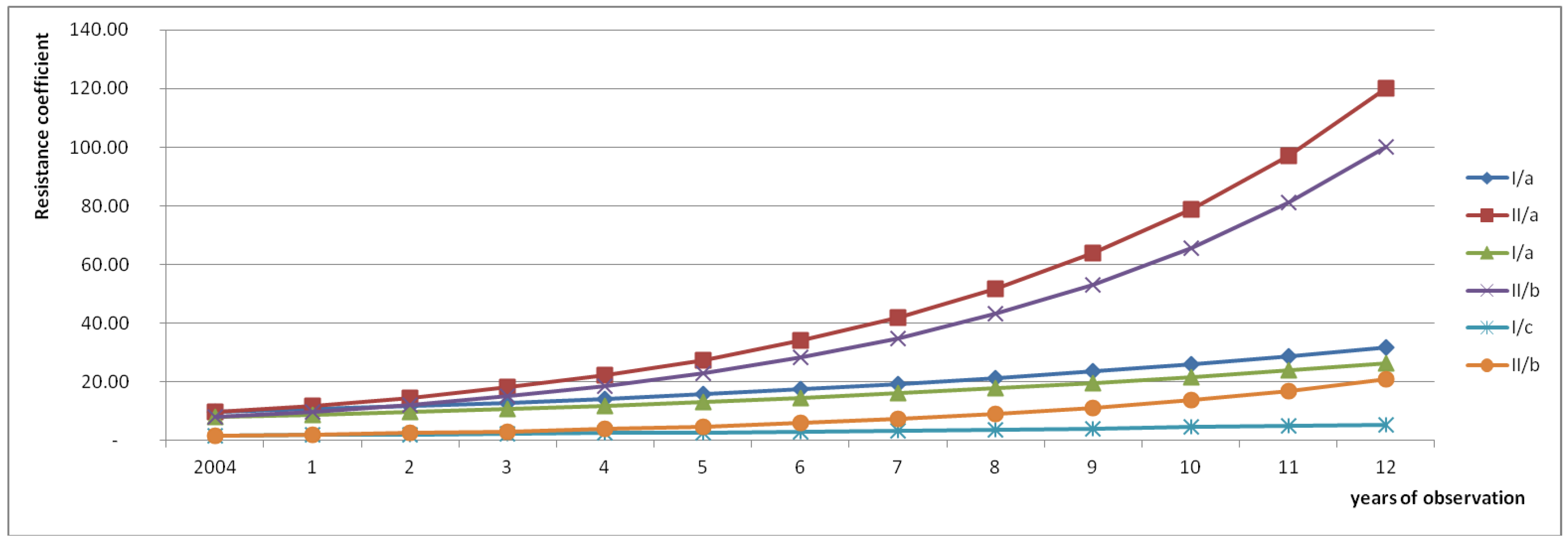
The parameter that more accurately describes the impact of shrubby vegetation on the water flow is the resistance coefficient. It takes into account the overlapping of disturbances caused by neighbouring plant elements (willow branches), as well as the ratio of water velocity reaching plant elements and the average velocity in the channel cross-section. The simulations of the resistance coefficient for scenarios I and II are included in Table 2. Regardless of the test zone and the chosen scenario, the value of the coefficient increased.
Figure 8 illustrates variability in the resistance coefficient (λ) within 12 years of simulation. With regard to scenario II considering zones a and b, the value of the resistance coefficient was three times higher than the value in other analysed cases.
As previously mentioned, the resistance coefficient depends on many parameters and therefore can take values from a wide range (Table 3).
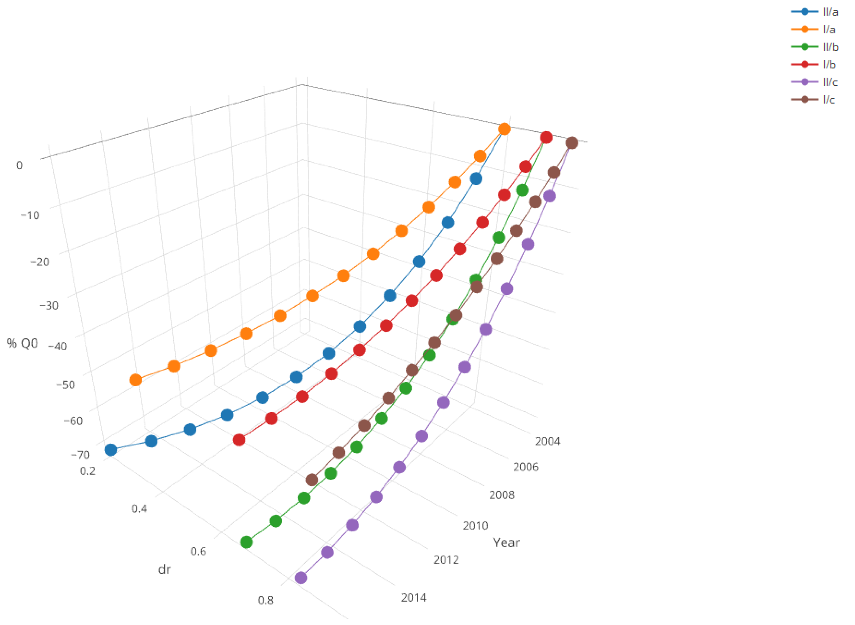
The parameter that takes into the consideration the geometrical dimensions of floodplain shrubby vegetation can be porosity. When its value is close to 1.0, it signals the possibility of the free passage of greater water flow. The information is of vital importance in case of high discharge. Figure 9 summarises the correlation between the share of voids in the vegetated cross-section and the loss of capacity of the analysed zones. The literature provides examples of numerous coefficients describing plant densities in river channels, e.g., the degree of development δR [64] determines the share of voids in the vegetated cross-section.
Analysing the results presented in Figure 9, it can be noted that the biggest reduction in flow occurred for scenario II, that is for the scenario in which the spacing was reduced while the diameter remained at a relatively constant level. In this case, the flow dropped by up to 70%. For scenario I, where the diameter changed, this decrease was recorded at the level of up to 45%. Han et al. [80] analyzed lateral velocity distribution in open channels with the use of elastic vegetation. They state that the vegetation can have a significant influence on the flow rate, reducing it by up to 70%. Thomas and Nisbet [81] indicate, in their research, that the planting of floodplain woodland could have a marked effect on flood flows. The additional roughness created by a complete cover of thick broadleaved woodland along the right bank of the floodplain increased flood water storage by 71% and delayed the downstream progression of the flood peak by 140 min.
The flow of water in floodplains is a very complicated process. It is affected by numerous factors related to both the morphology of floodplains and their hydraulic properties, i.e., landform, type, size and growth stage of vegetation, decrease in the water table, flow velocity, water depth, etc. Many of these factors are temporary or local. They might change across space and over time. Additionally, they can change over time cyclically (e.g. phases of plant development) or continuously. This variability may have a natural origin [82,83,84] (climate change) or results from anthropopression [85,86,87,88]. The quality of the hydrodynamic model used, e.g., for analysing flood wave transformation or flood risk management, can also be affected, apart from the purely physical factors discussed above, by other parameters, empirical coefficients included in the mathematical description of the flooding phenomenon, which are often taken a priori based on tables. The correct adoption of these parameters requires an appropriate procedure for tarring the model; however, it is also recommended that the parameter sensitivity and the parameter uncertainty be estimated [89], as well as the model’s sensitivity to changing parameters [90]. The sensitivity analysis should identify the key parameters that affect model performance. It also plays an important role in model parameterisation, calibration, optimisation, and uncertainty quantification [91,92]. Hydrodynamic models should not only take into consideration the spatial variability of parameters, but also their variation in time. Therefore, a systematic, periodic inspection of the analysed cross-section of the river should be carried out in order to update the numerical model used.
The sensitivity analysis of the model demonstrates that a double increase in diameter (in relation to the average diameter of 0.11) causes a change in the flow in the range of +25% for a two-fold reduction in diameter and about −23% for an increase in diameter. Similarly, a two-fold reduction or increase in the spacing between branches (in relation to the average value of 0.08 m) results in a flow change of −43% and +43%, respectively. This confirms that, for hydraulic reasons, it is much more important to maintain a proper spacing so as to ensure adequate flow during the passage of the flood wave.
Armanini et al. [93] indicated that the contribution of foliage (based on the prototype willow Salix alba) to global resistance of plants reaches 40% of total resistance. Research by Västilä et al. [94] indicated that the foliage-stem reference area ratio is an important controlling factor for the drag and frontal area reduction. The comparison results for foliated Black Poplars (P. nigra) to two Salix species suggest that the foliage–stem reference area ratio is an important factor explaining the between-species variation in flow resistance. Wilson et al. [95] also analysed the impact of foliage on the drag force of vegetation. The authors also examined the impact of foliage in terms of Manning-Strickler’s coefficient n. The ratio of Manning-Strickler’s coefficient n depends on the flow velocity and decreases with its increase. The higher the flow rate, the lower the effect of foliage on the flow resistance (in relation to leafless willows). For V = 0.2 ms−1 (designated during measurements for the flood in 2006), the increase in the coefficient n after taking into account the foliage for the willow group is about 2.2. Similar values were also obtained by Järvelä [96]. This causes a decrease in the flow, compared to the willow without leaves, by approx. 45% and of course depends on the flow rate. The higher the velocity, the lower the effect of foliage on the water flow rate.
4. Conclusions
Shrubby vegetation overgrowing floodplains (inter-embankment and polders) can have a significant impact on the capacity of the area in case of high discharge and/or flooding. It is noteworthy that the hydraulic characteristics of the river channel and floodplains dependent on, among other things, the existing vegetation, change over time, which is related to both the change in the vegetative phase of plants and the growth of plants in subsequent years.
The reference literature lacks extensive studies on the dynamics of growth of natural shrubby vegetation in the context of growth of diameter. Many literature items regarding willow growth concern biomass gain [72,97] and its height [72,98], in particular for energy purposes [99,100]. Even the most-recognized energy willow is affected by a large problem with obtaining reliable information about the growth rate, e.g., for different climate zones. All information on this subject is general, individual, and local. Therefore, numerical data can only be treated as estimated increments.
The field measurements consisting of the inventory of shrubby vegetation of the selected cross-sections carried out during the growing season within two following years allowed for performing simulations of their impact on the value of resistance and capacity of the floodplain areas. It should be noted that the analysed cross sections were characterised by vegetation occurring in various stages of growth, therefore, with different diameters and spacing of branches. The values of the diameter and spacing parameters are easy to define under both laboratory and field conditions. However, the selection of a representative area can be difficult, especially if there is a high spatial variability of vegetation. Additionally, considering the areas under cultivation, where systematic care treatments are carried out, the spatial variability of these values should be significantly smaller.
The article analysed shrubby vegetation growth over a 12-year period for three selected zones (a, b, c) and two scenarios (I, II). The first scenario (I) assumed that the vegetation was growing on the plot cultivated as an energy willow (common osier) plantation, whereas the second scenario (II) assumed that the plants were developing in an uncontrolled manner.
With regard to scenario II considering zones a and b, the value of the resistance coefficient was three times higher than the value in other analysed cases. In these cases, the flow dropped by up to 70%. In the case of controlled growth (willow plantation), the decrease of flow was recorded at the level of up to 45%.
Foliage (period of vegetation during a summer flood) of willow increases the flow resistance. Depending on the velocities, the ratio of Manning-Strickler’s coefficient nwith foliage/nwithout foliage varies from approx. 2 to 3 [95,96]. In the analyzed case, foliage reduced the flow by 45%, compared to the willow without leaves. In the case of scenario II, foliage may cause a decrease in the flow of up to 83%.
Willow is the most popular woody plant occurring in flood plains of rivers. Due to good climatic conditions (temperature, sun exposure, water availability), they can achieve significant biomass increments and are successfully used as energy crops. Cultivation of energy willows in floodplains, under controlled conditions (trim, care, etc.), might be finalized with economic benefits. The loss of free surface of high water flow imposes the necessity to maintain the area in good condition, inter alia by controlling the growth of vegetation. Maintenance works carried out by owners or tenants should be conducted consistently based on hydraulic and ecological knowledge.
For hydraulic reasons, floodplains should be planted with willow with a larger spacing than in the case of plantations. This is also confirmed by the sensitivity analysis. Therefore, the density of floodplain vegetations should be constantly monitored and depending on the management goals [101], such as maximising agricultural production, maximising biodiversity, or maximizing flood storage capacity, appropriately regulated (e.g., by increasing or decreasing vegetation density). Floodplain vegetation can be useful as a biological tool for the effective management of water quality, water routing, water resources, and restoring stream ecosystem [102]. Of course, it should not be forgotten that natural vegetation growing in an uncontrolled way can pose additional risk in the event of high water or impoundment.
Supplementary Materials
The following is available online at https://www.mdpi.com/2073-4441/10/5/556/s1, Figure 9 in an interactive form.
Author Contributions
N.W. contributed to the collection of data, preparation of data for simulation, and preparation of charts for the final presentation of results. Z.W. was responsible for data analysis and preparation of charts for the final presentation of results. T.K. contributed to the collection of data. M.H. formatted the text for the final publication. P.S. contributed to the presentation of the results. All co-authors took part in the writing process.
Conflicts of Interest
The authors declare no conflict of interest.
References
- Gurnell, A.M.; Bertoldi, W.; Corenblit, D. Changing river channels: The roles of hydrological processes, plants and pioneer fluvial landforms in humid temperate, mixed load, gravel bed rivers. Earth-Sci. Rev. 2012, 111, 129–141. [Google Scholar] [CrossRef]
- Crosato, A.; Saleh, M.S. Numerical study on the effects of floodplain vegetation on river planform style. Earth Surf. Process. Landf. 2011, 36, 711–720. [Google Scholar] [CrossRef]
- Tabacchi, E.; Correll, D.L.; Hauer, R.; Pinay, G.; Planty-Tabacchi, A.-M.; Wissmar, R.C. Development, maintenance and role of riparian vegetation in the river landscape. Freshw. Biol. 1998, 40, 497–516. [Google Scholar] [CrossRef]
- Murray, A.B.; Chris, P. Modelling the effect of vegetation on channel pattern in bedload rivers. Earth Surf. Process. Landf. 2003, 28, 131–143. [Google Scholar] [CrossRef]
- Schiechtl, H.M.; Stern, R. Naturnaher Wasserbau: Anleitung für Ingenieurbiologische Bauweisen; John Wiley & Sons: Berlin, Germany, 2002. [Google Scholar]
- Chen, S.-C.; Kuo, Y.-M.; Li, Y.-H. Flow characteristics within different configurations of submerged flexible vegetation. J. Hydrol. 2011, 398, 124–134. [Google Scholar] [CrossRef]
- Meire, D.W.; Kondziolka, J.M.; Nepf, H.M. Interaction between neighboring vegetation patches: Impact on flow and deposition. Water Resour. Res. 2014, 50, 3809–3825. [Google Scholar] [CrossRef] [Green Version]
- Bertoldi, W.; Welber, M.; Gurnell, A.M.; Mao, L.; Comiti, F.; Tal, M. Physical modelling of the combined effect of vegetation and wood on river morphology. Geomorphology 2015, 246, 178–187. [Google Scholar] [CrossRef]
- Nepf, H.M. Flow and transport in regions with aquatic vegetation. Ann. Rev. Fluid Mech. 2012, 44, 123–142. [Google Scholar] [CrossRef]
- Mazur, R.; Kałuża, T.; Chmist, J.; Walczak, N.; Laks, I.; Strzeliński, P. Influence of deposition of fine plant debris in river floodplain shrubs on flood flow conditions–The Warta River case study. Phys. Chem. Earth Parts A/B/C 2016, 94, 106–113. [Google Scholar] [CrossRef]
- Yang, P.-P.; Zhang, H.-L.; Ma, C. Effects of simulated submerged and rigid vegetation and grain roughness on hydraulic resistance to simulated overland flow. J. Mt. Sci. 2017, 14, 2042–2052. [Google Scholar] [CrossRef]
- Walczak, N.; Walczak, Z.; Hämmerling, M.; Przedwojski, B. Analytical model for vertical velocity distribution and hydraulic roughness at the flow through river bed and valley with vegetation. Rocznik Ochrona Środowiska 2013, 15, 405–419. [Google Scholar]
- Lee, J.K.; Roig, L.C.; Jenter, H.L.; Visser, H.M. Drag coefficients for modeling flow through emergent vegetation in the Florida Everglades. Ecol. Eng. 2004, 22, 237–248. [Google Scholar] [CrossRef]
- Zhao, M.; Fan, Z. Hydrodynamic characteristics of submerged vegetation flow with non-constant vertical porosity. PLoS ONE 2017, 12, e0176712. [Google Scholar] [CrossRef] [PubMed]
- Zeng, Y.; Huai, W.; Zhao, M. Flow characteristics of rectangular open channels with compound vegetation roughness. Appl. Math. Mech. 2016, 37, 341–348. [Google Scholar] [CrossRef]
- Jordanova, A.A.; James, C.S.; Birkhead, A.L. Practical estimation of flow resistance through emergent vegetation. Proc. Inst. Civ. Eng.-Water Manag. 2006, 159, 173–181. [Google Scholar] [CrossRef]
- Hui, E.-Q.; Hu, X.-E.; Jiang, C.-B.; Zhu, Z.-D. A study of drag coefficient related with vegetation based on the flume experiment. J. Hydrodyn. Ser. B 2010, 22, 329–337. [Google Scholar] [CrossRef]
- Aberle, J.; Järvelä, J. Flow resistance of emergent rigid and flexible floodplain vegetation. J. Hydraul. Res. 2013, 51, 33–45. [Google Scholar] [CrossRef]
- Miyab, N.M.; Afzalimehr, H.; Singh, V.P.; Ghorbani, B. On Flow Resistance Due to Vegetation in a Gravel-Bed River. Int. J. Hydraul. Eng. 2014, 3, 85–92. [Google Scholar]
- Gurnell, A. Plants as river system engineers. Earth Surf. Process. Landf. 2014, 39, 4–25. [Google Scholar] [CrossRef]
- Uijttewaal, W.S.J. Hydrodynamics of shallow flows: Application to rivers. J. Hydraul. Res. 2014, 52, 157–172. [Google Scholar] [CrossRef]
- Verschoren, V.; Meire, D.; Schoelynck, J.; Buis, K.; Bal, K.D.; Troch, P.; Meire, P.; Temmerman, S. Resistance and reconfiguration of natural flexible submerged vegetation in hydrodynamic river modelling. Environ. Fluid Mech. 2016, 16, 245–265. [Google Scholar] [CrossRef] [Green Version]
- Meitzen, K.M.; Phillips, J.N.; Perkins, T.; Manning, A.; Julian, J.P. Catastrophic flood disturbance and a community’s response to plant resilience in the heart of the Texas Hill Country. Geomorphology 2018, 305, 20–32. [Google Scholar] [CrossRef]
- Ishikawa, Y.; Sakamoto, T.; Mizuhara, K. Effect of density of riparian vegetation on effective tractive force. J. For. Res. 2003, 8, 235–246. [Google Scholar] [CrossRef]
- Gu, F.-F.; Ni, H.-G.; Qi, D.-M. Roughness coefficient for unsubmerged and submerged reed. J. Hydrodyn. Ser. B 2007, 19, 421–428. [Google Scholar] [CrossRef]
- Zhang, M.; Li, C.W.; Shen, Y. Depth-averaged modeling of free surface flows in open channels with emerged and submerged vegetation. Appl. Math. Model. 2013, 37, 540–553. [Google Scholar] [CrossRef]
- Aberle, J.; Järvelä, J. Hydrodynamics of vegetated channels. In Rivers—Physical, Fluvial and Environmental Processes; Rowinski, P., Radecki-Pawlik, A., Eds.; Springer International Publishing: Cham, Switzerland, 2015; pp. 519–541. [Google Scholar]
- Gran, K.; Paola, C. Riparian vegetation controls on braided stream dynamics. Water Resour. Res. 2001, 37, 3275–3283. [Google Scholar] [CrossRef]
- Politti, E.; Bertoldi, W.; Gurnell, A.; Henshaw, A. Feedbacks between the riparian Salicaceae and hydrogeomorphic processes:A quantitative review. Earth-Sci. Rev. 2018, 176, 147–165. [Google Scholar] [CrossRef]
- Merritt, D.M.; Scott, M.L.; Leroy Poff, N.; Auble, G.T.; Lytle, D.A. Theory, methods and tools for determining environmental flows for riparian vegetation: Riparian vegetation-flow response guilds. Freshw. Biol. 2010, 55, 206–225. [Google Scholar] [CrossRef]
- Nilsson, C.; Berggren, K. Alterations of riparian ecosystems caused by river regulation: Dam operations have caused global-scale ecological changes in riparian ecosystems. How to protect river environments and human needs of rivers remains one of the most important questions of our time. BioScience 2000, 50, 783–792. [Google Scholar]
- Bätz, N.; Colombini, P.; Cherubini, P.; Lane, S.N. Groundwater controls on biogeomorphic succession and river channel morphodynamics. J. Geophys. Res. Earth Surf. 2016, 121, 1763–1785. [Google Scholar] [CrossRef]
- Gullberg, U. Towards making willows pilot species for coppicing production. For. Chron. 1993, 69, 721–726. [Google Scholar] [CrossRef]
- Haughton, A.J.; Bond, A.J.; Lovett, A.A.; Dockerty, T.; Sünnenberg, G.; Clark, S.J.; Bohan, D.A.; Sage, R.B.; Mallott, M.D.; Mallott, V.E.; et al. A novel, integrated approach to assessing social, economic and environmental implications of changing rural land-use: A case study of perennial biomass crops. J. Appl. Ecol. 2009, 46, 315–322. [Google Scholar] [CrossRef]
- Lisowski, A. Technologie Zbioru Roślin Energetycznych; Wydawnictwo SGGW: Warsaw, Poland, 2010. (In Polish) [Google Scholar]
- Dubas, J.W.; Grzybek, A.; Kotowski, W.; Tomczyk, A. Wierzba Energetyczna—Uprawa i Technologie Przetwarzania; Wyższa Szkoła Ekonomii i Administracji w Bytomiu: Bytom, Poland, 2004; Volume 35. [Google Scholar]
- Bullard, M.J.; Mustill, S.J.; McMillan, S.D.; Nixon, P.M.I.; Carver, P.; Britt, C.P. Yield improvements through modification of planting density and harvest frequency in short rotation coppice Salix spp.—1. Yield response in two morphologically diverse varieties. Biomass Bioenergy 2002, 22, 15–25. [Google Scholar] [CrossRef]
- Melin, G.; Larsson, S. Agrobränsle AB—world leading company on short rotation coppice willow. In Proceedings of the 14th European Biomass Conference, Paris, France, 17–21 October 2005; pp. 36–37. [Google Scholar]
- Hoffmann, D.; Weih, M. Limitations and improvement of the potential utilisation of woody biomass for energy derived from short rotation woody crops in Sweden and Germany. Biomass Bioenergy 2005, 28, 267–279. [Google Scholar] [CrossRef]
- Mola-Yudego, B.; Pelkonen, P. The effects of policy incentives in the adoption of willow short rotation coppice for bioenergy in Sweden. Energy Policy 2008, 36, 3062–3068. [Google Scholar] [CrossRef]
- Kopp, R.F.; Abrahamson, L.P.; White, E.H.; Volk, T.A.; Nowak, C.A.; Fillhart, R.C. Willow biomass production during ten successive annual harvests. Biomass Bioenergy 2001, 20, 1–7. [Google Scholar] [CrossRef]
- Liro, A.; Tederko, Z. Strategia Wdrażania Krajowej Sieci Ekologicznej ECONET-Polska: Praca Zbiorowa; Fundacja IUCN Poland: Warsaw, Poland, 1998. [Google Scholar]
- BirdLife Data Zone. Available online: http://datazone.birdlife.org/site/factsheet/926 (accessed on 10 April 2018).
- Straatsma, M.W.; Middelkoop, H. Airborne laser scanning as a tool for lowland floodplain vegetation monitoring. Hydrobiologia 2006, 565, 87–103. [Google Scholar] [CrossRef]
- Tymiński, T. Hydraulic Model Investigation of Flow Conditions for Floodplains with Coniferous and Deciduous Shrubs. Pol. J. Environ. Stud. 2012, 21, 1047–1052. [Google Scholar]
- Ballesteros, J.A.; Bodoque, J.M.; Díez-Herrero, A.; Sanchez-Silva, M.; Stoffel, M. Calibration of floodplain roughness and estimation of flood discharge based on tree-ring evidence and hydraulic modelling. J. Hydrol. 2011, 403, 103–115. [Google Scholar] [CrossRef]
- Anderson, B.G.; Rutherfurd, I.D.; Western, A.W. An analysis of the influence of riparian vegetation on the propagation of flood waves. Environ. Model. Softw. 2006, 21, 1290–1296. [Google Scholar] [CrossRef]
- Zong, L.; Nepf, H. Flow and deposition in and around a finite patch of vegetation. Geomorphology 2010, 116, 363–372. [Google Scholar] [CrossRef]
- Ortiz, A.C.; Ashton, A.; Nepf, H. Mean and turbulent velocity fields near rigid and flexible plants and the implications for deposition. J. Geophys. Res. Earth Surf. 2013, 118, 2585–2599. [Google Scholar] [CrossRef]
- Vargas-Luna, A.; Crosato, A.; Uijttewaal, W.S.J. Effects of vegetation on flow and sediment transport: Comparative analyses and validation of predicting models. Earth Surf. Process. Landf. 2015, 40, 157–176. [Google Scholar] [CrossRef]
- Wu, F.-S. Characteristics of Flow Resistance in Open Channels with Non-Submerged Rigid Vegetation. J. Hydrodyn. Ser. B 2008, 20, 239–245. [Google Scholar] [CrossRef]
- Thorne, C.R. Effects of vegetation on riverbank erosion and stability. In Vegetation and Erosion: Processes and Environments; John Wiley: Chichester, UK, 1990; pp. 125–144. [Google Scholar]
- Florsheim, J.L.; Mount, J.F.; Chin, A. Bank erosion as a desirable attribute of rivers. AIBS Bull. 2008, 58, 519–529. [Google Scholar] [CrossRef]
- Wang, H.; Tang, H.-W.; Zhao, H.-Q.; Zhao, X.-Y.; Lü, S.-Q. Incipient motion of sediment in presence of submerged flexible vegetation. Water Sci. Eng. 2015, 8, 63–67. [Google Scholar] [CrossRef]
- Västilä, K.; Järvelä, J. Characterizing natural riparian vegetation for modeling of flow and suspended sediment transport. J. Soils Sediments 2017, 1–17. [Google Scholar] [CrossRef]
- Walczak, N.; Walczak, Z.; Hämmerling, M.; Spychala, M.; Niec, J. Head Losses in Small Hydropower Plant Trash Racks (SHP). Acta Sci. Pol. Form. Circumiectus 2016, 15, 369–382. [Google Scholar]
- Vries, P.G. Sampling Theory for Forest Inventory: A Teach-Yourself Course; Springer: Berlin/Heidelberg, Germany, 1986. [Google Scholar]
- Kałuża, T. Einfluss der Bewuchsentwicklung auf das Abflussverhalten in Fliessgewassern. Wasserwirtschaft 2009, 99, 29–32. [Google Scholar]
- Juliszewski, T.; Kwaśniewski, D.; Baran, D. Comparison of planting of energetic willow (salix viminalis) in the spring and autumn time. Inżynieria Rolnicza 2005, 9, 251–258. (In Polish) [Google Scholar]
- Rickert, K. Der Einfluß von Gehölzen auf die Lichtverhältnisse und das Abflußverhalten in Fließgewässern; Institut für Wasserwirtschaft, Hydrologie und Landwirtschaftlichen Wasserbau: Hannover, Germany, 1986. (In German) [Google Scholar]
- Kubrak, J.; Kozioł, A.; Kubrak, E.; Wasilewicz, M.; Kiczko, A. Analiza wpływu roślinności na warunki przepływu wody w międzywalu. In Określenie Kryteriów Ustalania Miejsc Przeprowadzania Wycinek i Usuwania Nadmiaru Roślinności. Szkoła Główna Gospodarstwa Wiejskiego w Warszawie; Wydział Budownictwa i Inżynierii Środowiska: Warsaw, Poland, 2012. [Google Scholar]
- Tworkowski, J.; Szczukowski, S.; Stolarski, M. Yielding and morphological characteristics of willow grown in eco-salix system. Fragm. Agron. 2010, 27, 135–146. [Google Scholar]
- Kubrak, J.; Nachlik, E. Hydrauliczne Podstawy Obliczania Przepustowości Koryt Rzecznych; Wydawnictwo SGGW: Warsaw, Poland, 2003. (In Polish) [Google Scholar]
- Lindner, K. Der Strömungswiderstand von Pflanzenbeständen. Mitteilungen 75; Leichtweiss-Institut für Wasserbau, Technische Universität Braunschweig: Braunschweig, Germany, 1982. (In German) [Google Scholar]
- Pasche, E. Turbulenzmechanismen in Naturnahen Fließgewässern und Die Möglichkeit Ihrer Mathematischen Erfassung; Lehrstuhl und Institut für Wasserbau und Wasserwirtschaft: Aachen, Germany, 1984. (In German) [Google Scholar]
- Jovanovic, M.; Pasche, E.; Töppel, M.; Donner, M. 1D-Hydraulic; Technische Universität: Hamburg, Germany, 2006. [Google Scholar]
- Deutscher Verband für Wasserwirtschaft und Kulturbau (DVWK). Hydraulische Berechnung von Fließgewässern; DVWK Merkblätter zur Wasserwirtschaft; Paul Parey: Berlin, Germany, 1991. (In German) [Google Scholar]
- Rickert, K.; Nickel, A. Naturnahe Regelung von Fließgewässern; Unterlagen zum Kurs WH06 des Weiterbildungsstudiums “Wasser und Umwelt” der; Universität Hannover: Hanover, Germany, 2003. (In German) [Google Scholar]
- Stolarski, M.; Kisiel, R.; Szczukowski, S.; Tworkowski, J. Costs of liquidation of short-rotation willow plantation. Roczniki Nauk Rolniczych Seria G 2008, 94, 172–177. (In Polish) [Google Scholar]
- Wrócił Czas Wierzby Energetycznej!—Agrofakt.pl. Available online: https://www.agrofakt.pl/czas-wierzby-energetycznej/ (accessed on 12 April 2018).
- Szczukowski, S.; Budny, J. Wierzba Krzewiasta-Roślina Energetyczna; Wojewódzki Fundusz Ochrony Środowiska i Gospodarki Wodnej: Olsztyn, Poland, 2003. [Google Scholar]
- Stolarski, M.J.; Szczukowski, S.; Tworkowski, J.; Klasa, A. Willow biomass production under conditions of low-input agriculture on marginal soils. For. Ecol. Manag. 2011, 262, 1558–1566. [Google Scholar] [CrossRef]
- Zaliwski, A.S. Technological and organizational aspects of combining agricultural production for food and energy. Agric. Eng. 2013, 4, 399–407. (In Polish) [Google Scholar]
- Szczukowski, S.; Tworkowski, J.; Wiwart, M.; Przyborowski, J. Wiklina (Salix sp.) Uprawa i Możliwości Wykorzystania; Wydawnictwo Uniwersytetu Warmińsko-Mazurskiego: Olsztyn, Poland, 2002. [Google Scholar]
- Swiatek, D.; Wej, A. The computer program RIVER for calculation of the flow capacity of the vegetated river valley. Infrastruktura i Ekologia Terenów Wiejskich 2006, 4, 173–182. (In Polish) [Google Scholar]
- Miroslaw-Swiatek, D.; Amatya, D.M. Effects of cypress knee roughness on flow resistance and discharge estimates of the Turkey Creek watershed. Ann. Wars. Univ. Life Sci. SGGW. Land Reclam. 2017, 49, 179–199. [Google Scholar] [CrossRef]
- Da Silva, Y.J.A.B.; Cantalice, J.R.B.; Singh, V.P.; Cruz, C.M.C.A.; Silva Souza, W.L.D. Sediment transport under the presence and absence of emergent vegetation in a natural alluvial channel from Brazil. Int. J. Sediment Res. 2016, 31, 360–367. [Google Scholar] [CrossRef]
- Romero, M.; Revollo, N.; Molina, J. Flow resistance in steep mountain rivers in Bolivia. J. Hydrodyn. Ser. B 2010, 22, 702–707. [Google Scholar] [CrossRef]
- Gilley, J.E.; Kottwitz, E.R.; Wieman, G.A. Darcy-Weisbach roughness coefficients for gravel and cobble surfaces. J. Irrig. Drain. Eng. 1992, 118, 104–112. [Google Scholar] [CrossRef]
- Han, L.; Zeng, Y.; Chen, L.; Huai, W. Lateral velocity distribution in open channels with partially flexible submerged vegetation. Environ. Fluid Mech. 2016, 16, 1267–1282. [Google Scholar] [CrossRef]
- Thomas, H.; Nisbet, T.R. An assessment of the impact of floodplain woodland on flood flows. Water Environ. J. 2007, 21, 114–126. [Google Scholar] [CrossRef]
- Billi, P.; Fazzini, M. Global change and river flow in Italy. Glob. Planet. Chang. 2017, 155, 234–246. [Google Scholar] [CrossRef]
- Marchese, E.; Scorpio, V.; Fuller, I.; McColl, S.; Comiti, F. Morphological changes in Alpine rivers following the end of the Little Ice Age. Geomorphology 2017, 295, 811–826. [Google Scholar] [CrossRef]
- Arnaud-Fassetta, G. River channel changes in the Rhone Delta (France) since the end of the Little Ice Age: Geomorphological adjustment to hydroclimatic change and natural resource management. Catena 2003, 51, 141–172. [Google Scholar] [CrossRef]
- Comiti, F.; Da Canal, M.; Surian, N.; Mao, L.; Picco, L.; Lenzi, M.A. Channel adjustments and vegetation cover dynamics in a large gravel bed river over the last 200 years. Geomorphology 2011, 125, 147–159. [Google Scholar] [CrossRef]
- Chin, A. Urban transformation of river landscapes in a global context. Geomorphology 2006, 79, 460–487. [Google Scholar] [CrossRef]
- Magilligan, F.J.; Nislow, K.H. Changes in hydrologic regime by dams. Geomorphology 2005, 71, 61–78. [Google Scholar] [CrossRef]
- Gregory, K.J. The human role in changing river channels. Geomorphology 2006, 79, 172–191. [Google Scholar] [CrossRef]
- Benke, K.K.; Lowell, K.E.; Hamilton, A.J. Parameter uncertainty, sensitivity analysis and prediction error in a water-balance hydrological model. Math. Comput. Model. 2008, 47, 1134–1149. [Google Scholar] [CrossRef]
- Zhan, C.-S.; Song, X.-M.; Xia, J.; Tong, C. An efficient integrated approach for global sensitivity analysis of hydrological model parameters. Environ. Model. Softw. 2013, 41, 39–52. [Google Scholar] [CrossRef]
- Song, X.; Zhang, J.; Zhan, C.; Xuan, Y.; Ye, M.; Xu, C. Global sensitivity analysis in hydrological modeling: Review of concepts, methods, theoretical framework, and applications. J. Hydrol. 2015, 523, 739–757. [Google Scholar] [CrossRef]
- Castaings, W.; Dartus, D.; Le Dimet, F.-X.; Saulnier, G.-M. Sensitivity analysis and parameter estimation for distributed hydrological modeling: Potential of variational methods. Hydrol. Earth Syst. Sci. 2009, 13, 503–517. [Google Scholar] [CrossRef] [Green Version]
- Armanini, A.; Righetti, M.; Grisenti, P. Direct measurement of vegetation resistance in prototype scale. J. Hydraul. Res. 2005, 43, 481–487. [Google Scholar] [CrossRef]
- Västilä, K.; Järvelä, J.; Aberle, J. Characteristic reference areas for estimating flow resistance of natural foliated vegetation. J. Hydrol. 2013, 492, 49–60. [Google Scholar] [CrossRef]
- Wilson, C.A.; Hoyt, J.; Schnauder, I. Impact of foliage on the drag force of vegetation in aquatic flows. J. Hydraul. Eng. 2008, 134, 885–891. [Google Scholar] [CrossRef]
- Järvelä, J. Flow resistance of flexible and stiff vegetation: A flume study with natural plants. J. Hydrol. 2002, 269, 44–54. [Google Scholar] [CrossRef]
- Searle, S.Y.; Malins, C.J. Will energy crop yields meet expectations? Biomass Bioenergy 2014, 65, 3–12. [Google Scholar] [CrossRef]
- Bilyeu, D.M.; Cooper, D.J.; Hobbs, N.T. Water tables constrain height recovery of willow on Yellowstone’s northern range. Ecol. Appl. 2008, 18, 80–92. [Google Scholar] [CrossRef] [PubMed]
- Toivonen, R.M.; Tahvanainen, L.J. Profitability of willow cultivation for energy production in Finland. Biomass Bioenergy 1998, 15, 27–37. [Google Scholar] [CrossRef]
- Ericsson, K.; Rosenqvist, H.; Ganko, E.; Pisarek, M.; Nilsson, L. An agro-economic analysis of willow cultivation in Poland. Biomass Bioenergy 2006, 30, 16–27. [Google Scholar] [CrossRef]
- Posthumus, H.; Rouquette, J.R.; Morris, J.; Gowing, D.J.G.; Hess, T.M. A framework for the assessment of ecosystem goods and services; a case study on lowland floodplains in England. Ecol. Econ. 2010, 69, 1510–1523. [Google Scholar] [CrossRef]
- Tabacchi, E.; Lambs, L.; Guilloy, H.; Planty-Tabacchi, A.-M.; Muller, E.; Dcamps, H. Impacts of riparian vegetation on hydrological processes. Hydrol. Process. 2000, 14, 2959–2976. [Google Scholar] [CrossRef]
Figure 1.
Place for measuring diameters and spacing.

Figure 2.
Case study system-reach of Warta River.

Figure 3.
Simulation diagram of the vegetation grown on the plot during 12 years of observation.

Figure 4.
Simulation diagram of the vegetation grown uncontrollably at the beginning (2004) and the end (2016) of observations.
Figure 4.
Simulation diagram of the vegetation grown uncontrollably at the beginning (2004) and the end (2016) of observations.

Figure 5.
Variability in the diameter values depending on age. Own study based on the authors' data and [58].
Figure 5.
Variability in the diameter values depending on age. Own study based on the authors' data and [58].

Figure 6.
Variability in the diameter of branches occurring during years of simulation.

Figure 7.
Variability in the spacing between branches in both directions of flow in years.

Figure 8.
Variability in the resistance coefficient during 2004–2016.

Figure 9.
Percentage change in the capacity of floodplain areas for the analysed scenarios and test zones. Supplementary Materials include Figure 9 in an interactive form.
Figure 9.
Percentage change in the capacity of floodplain areas for the analysed scenarios and test zones. Supplementary Materials include Figure 9 in an interactive form.


Table 1.
Standard deviations (SD) and coefficient variations (Cv) of the diameter and distance value.
Table 1.
Standard deviations (SD) and coefficient variations (Cv) of the diameter and distance value.
| Parameter | Diameter | Distance | ||
|---|---|---|---|---|
| zone | SD | Cv | SD | Cv |
| I/a | 0.014 | 0.366 | 0.001 | 0.008 |
| II/a | 0.002 | 0.077 | 0.022 | 0.366 |
| I/b | 0.004 | 0.366 | 0.000 | 0.008 |
| II/b | 0.001 | 0.077 | 0.013 | 0.366 |
| I/c | 0.005 | 0.366 | 0.001 | 0.008 |
| II/c | 0.010 | 0.530 | 0.026 | 0.366 |
Table 2.
Change in the resistance coefficient for the analysed scenarios in three test zones.
| Option/Zone | Years of Obsrevation | ||||||||||||
|---|---|---|---|---|---|---|---|---|---|---|---|---|---|
| 0 | 1 | 2 | 3 | 4 | 5 | 6 | 7 | 8 | 9 | 10 | 11 | 12 | |
| Resistance Coefficient (-) | |||||||||||||
| I/a | 9.66 | 10.66 | 11.77 | 12.99 | 14.34 | 15.83 | 17.48 | 19.30 | 21.31 | 23.53 | 25.98 | 28.68 | 31.67 |
| II/a | 9.66 | 11.91 | 14.68 | 18.11 | 22.33 | 27.55 | 33.99 | 41.94 | 51.74 | 63.85 | 78.79 | 97.23 | 119.98 |
| I/b | 8.06 | 8.90 | 9.82 | 10.84 | 11.96 | 13.20 | 14.58 | 16.09 | 17.77 | 19.61 | 21.66 | 23.91 | 26.40 |
| II/b | 8.06 | 9.93 | 12.25 | 15.10 | 18.62 | 22.97 | 28.34 | 34.96 | 43.13 | 53.22 | 65.67 | 81.03 | 99.99 |
| I/c | 1.73 | 1.90 | 2.09 | 2.31 | 2.54 | 2.80 | 3.08 | 3.40 | 3.75 | 4.13 | 4.56 | 5.03 | 5.55 |
| II/c | 1.73 | 2.12 | 2.60 | 3.19 | 3.93 | 4.83 | 5.95 | 7.33 | 9.03 | 11.13 | 13.73 | 16.93 | 20.88 |
Table 3.
Summary of resistance coefficients based on literature.
| Author | The Scope of the Study | The Range of Dimensionless Resistance Coefficient |
|---|---|---|
| Kałuża [58] | Ems-field measurements | 0.08–0.175 |
| Swiatek, D., and Wej, A. [75] | Biebrza-field measurements | 0.04–1.424 |
| Miroslaw-Swiatek, D., and Amatya, D.M. [76] | Turcja-field measurements | 0.15–0.47 |
| da Silva, et al. [77] | Brazil-field measurements | 0.38–47.67 |
| Mauricio Romero et al. [78] | Bolivia-field measurements, Riverbed slope | 0.18–7.0 |
| Gilley et al. [79] | Laboratory | 0.1–8.0 |
© 2018 by the authors. Licensee MDPI, Basel, Switzerland. This article is an open access article distributed under the terms and conditions of the Creative Commons Attribution (CC BY) license (http://creativecommons.org/licenses/by/4.0/).
Share and Cite
MDPI and ACS Style
Walczak, N.; Walczak, Z.; Kałuża, T.; Hämmerling, M.; Stachowski, P. The Impact of Shrubby Floodplain Vegetation Growth on the Discharge Capacity of River Valleys. Water 2018, 10, 556. https://doi.org/10.3390/w10050556
AMA Style
Walczak N, Walczak Z, Kałuża T, Hämmerling M, Stachowski P. The Impact of Shrubby Floodplain Vegetation Growth on the Discharge Capacity of River Valleys. Water. 2018; 10(5):556. https://doi.org/10.3390/w10050556
Chicago/Turabian StyleWalczak, Natalia, Zbigniew Walczak, Tomasz Kałuża, Mateusz Hämmerling, and Piotr Stachowski. 2018. "The Impact of Shrubby Floodplain Vegetation Growth on the Discharge Capacity of River Valleys" Water 10, no. 5: 556. https://doi.org/10.3390/w10050556
Note that from the first issue of 2016, this journal uses article numbers instead of page numbers. See further details here.