Article

Evapotranspiration Partition and Crop Coefficients of Tifton 85 Bermudagrass as Affected by the Frequency of Cuttings. Application of the FAO56 Dual Kc Model

1
Centro de Investigação em Agronomia, Alimentos, Ambiente e Paisagem (LEAF), Instituto Superior de Agronomia, Universidade de Lisboa, Tapada da Ajuda, 1349-017 Lisboa, Portugal
2
Centro de Ciências Rurais, Universidade Federal de Santa Maria, Cidade Universitária, Bairro Camobi, 97105-900 Santa Maria, RS, Brazil
*
Author to whom correspondence should be addressed.
Water 2018, 10(5), 558; https://doi.org/10.3390/w10050558
Submission received: 21 March 2018 / Revised: 23 April 2018 / Accepted: 23 April 2018 / Published: 26 April 2018
(This article belongs to the Special Issue Innovation Issues in Water, Agriculture and Food)

Abstract

:
This study aims to model the impacts of the frequency of cuttings of Tifton 85 bermudagrass on the dynamics of evapotranspiration (ETc) and to derive crop coefficients appropriate for grass water management. Two seasons of experimentation were used with four different cutting treatments which provided field data for calibration and validation of the soil water balance model SIMDualKc for all treatments. Cuttings were performed after the cumulative growth degree days (CGDD) attained 124 °C, 248 °C and 372 °C, thus from short to very long intervals between cuttings. SIMDualKc adopts the Food and Agriculture Organization (FAO) dual Kc approach for partitioning ET into crop transpiration and soil evaporation, thus providing for an assessment of their dynamics. All treatments were irrigated to avoid water stress. Grass ETc was modelled adopting a Kcb curve to describe the ET variation for each cutting cycle, that is, using the FAO Kc curve that consists of a series of Kcb curves relative to each cutting cycle. Each individual Kcb curve consisted of three segments constructed when knowing the Kcb values at the initial, at the end of rapid growth, and at cutting, respectively Kcb ini, Kcb gro and Kcb cut. These Kcb values were first estimated using the equation relating Kcb to the density coefficient (Kd), which is computed from the fraction of ground cover (fc) and canopy height (h) at the same dates. The goodness of fit indicators relative to the calibration and validation of the SIMDualKc model were rather good, with the normalized root mean square error (RMSE) ranging from 4.0% to 6.7% of the mean available soil water. As an example, the standard Kcb values obtained after model calibration relative to the cuttings treatment with CGDD of 248 °C are: Kcb ini = 0.86, Kcb gro = 0.91 and Kcb cut = 0.96. Kcb values were smaller when the frequency of cuts was larger because h and fc were smaller, and were larger for reduced cuttings frequency since h and fc were then larger. Because the soil was wet most of the time, the soil evaporation Ke varied little but its value was small due to the combined effects of the fraction of crop cover and plant litter covering the soil. The values of Kc = Kcb+Ke also varied little due to the influence of Ke and the Kc curve obtained a form different from the Kcb curves, and a single Kc value was adopted for each cutting frequency, e.g., Kc = 0.99 for the treatment with CGDD of 248 °C. Results of the soil water balance have shown that, during the experimental periods, likely due to the effects of the El Niño Southern Oscillation (ENSO), runoff and deep percolation exceeded ETc. Moreover, the soil evaporation ratio was small: 14% in case of frequent cuttings and less for more spaced cuttings, thus with a transpiration ratio close to 90%, which indicates a very high beneficial consumptive water use, mainly when cuttings are not very frequent.

1. Introduction

The landscape of southern Brazil is characterized by the Pampa biome, which occupies 63% of the State of Rio Grande do Sul. Grassland is the dominant vegetation and livestock production is a main economic activity in the area, but large areas have been converted into cropland, mainly for soybean production, thus suppressing the native grass vegetation [1]. Therefore, the sustainability of this biome for livestock production requires the planting of new and highly productive grasses such as the Tifton 85 bermudagrass [2,3], recently introduced in the region. Assessing grass evapotranspiration and water requirements as influenced by the frequency of cuttings is required to support an upgraded management of those grasslands. An innovative approach used is to relate the frequency of cuttings with the density coefficient (Kd) and then estimate the basal crop coefficient from Kd following the Allen and Pereira approach [4].
Studies on evapotranspiration (ET) of grasslands are numerous. Research has commonly been devoted to assessing the dynamics and abiotic driving factors of ET, mainly relative to climate influences on the processes of energy partition into latent and sensible heat. Such studies often use eddy covariance and/or Bowen ratio energy balance (BREB) observations, data which are commonly used in analysis performed with the Penman–Monteith (PM) combination equation [5] and/or the Priestley–Taylor (PT) equation [6], thus using the canopy resistance or the PT parameter α as behavioral indicators [7,8,9]. As an alternative to those measurement techniques, scintillometer measurements [10] and satellite images [11,12,13] were also used. Adopting similar research approaches, other studies compared the ET of grasslands with ET of forests or shrublands [14,15,16]. In addition to the available energy for evaporation, soil water availability and crop ground cover or the leaf area index (LAI) were often identified as main driving factors influencing grass ET [14,15,16,17].
Studies such as those referred to above are likely of great importance for understanding the variability of grass ET when focusing on the Pampa biome but different, operational research approaches are required when aiming at knowing grassland water requirements and/or grassland water management issues. Related operational studies are also numerous and refer to various climates, grass species and diverse herbage uses for hay or for grazing with different frequency of cuttings. However, such ET studies are lacking in southern Brazil and for Tifton 85 bermudagrass. ET research aiming at improved farm water management generally uses the grass reference ET (ETo) proposed in the Food and Agriculture Organization guidelines for computing crop water requirements (FAO56) [17]; nevertheless, recent studies [3,18] relative to irrigated bermudagrass yields used the climatic potential ET equation of Thornthwaite [19], developed in 1948.
The reference ETo was defined after parameterizing the PM combination equation [5] for a cool season grass, thus resulting that ETo is defined as the rate of evapotranspiration from a hypothetical reference crop with an assumed crop height h = 0.12 m, a fixed daily canopy resistance rs = 70 s m−1, and an albedo of 0.23, closely resembling the evapotranspiration from an extensive surface of green grass of uniform height, actively growing, completely shading the ground and not short of water [17]. This definition is described by the daily PM-ETo equation [17], which represents the climatic demand of the atmosphere. Thus, following FAO56 [17], the ETo is to be used with a crop coefficient (Kc) when estimating or predicting the ET of a given surface, that is, the Kc-ETo approach. Kc is the ratio between the crop ET and ETo and varies with the crop surface characteristics and the crop growth stage, and is influenced by the climate and management. Single and dual Kc may be used [17]. The dual Kc consists of the sum Ke + Kcb of the soil evaporation coefficient (Ke) and the basal crop coefficient (Kcb), and thus with consideration of both processes included in evapotranspiration. The Kc values are standard or potential when the crop is not stressed, while actual Kc values (Kc act or Kcb act) are often smaller than the standard Kc or Kcb when water, salt, disease or management stresses affect crop transpiration. These effects may be considered using a stress coefficient applied to Kc or Kcb. Tabulated values of standard Kc and Kcb are provided by Allen et al. [17] for a variety of crops, including grasses and pastures. The standard Kc and Kcb values are transferable to other sites considering adjustments for climate described by Allen et al. [17]. The time variation of the Kc and Kcb values are described by Kc curves [17] that describe in a simplified way the dynamics of LAI and vegetation ET. The form of these curves varies from one crop to another; for grasses with cuttings, several successive Kc curves should be considered, each representing the dynamics of ET during each crop growth cycle between cuttings [17].
The operational use of the ETo equation implies, therefore, the use of crop coefficients and the build-up of Kc curves to describe the respective time variation. It could be observed that several papers reporting on the use of the grass reference ETo did not follow the concepts described above. A few authors directly compared ET obtained with eddy covariance, BREB, or a soil water balance with ETo but not searching for a Kc value [20], or even assumed equality between grass ET and ETo [21]. Other authors just computed daily Kc act values (often using different designations for that parameter) but did not search for a Kc curve that would describe their seasonal variation [22,23], or just identified a mean seasonal Kc act [24]. The lack of search for a Kc curve led some authors to consider the Kc-ETo approach as non-useful [25]. By contrast, Pronger et al. [26] did not clearly assume the concepts behind actual vs. potential Kc and, in addition to Ks, adopted a correction factor to ETo for highly stressed grass. This is theoretically not appropriate because it contradicts the concepts of reference ET, which depends solely upon the climate and not the crop under study, and of the Kc act that has to be derived from the standard Kc when adapting to the management and environmental conditions [17]. The approaches referred to above, like other research quoted before, may support an improved understanding of the dynamic behaviour of grass ET but are likely not appropriate for operational use in irrigation water management.
The FAO56 Kc-ETo method [17] was first applied by Cancela et al. [27] to grass using the single Kc act with successive four-stage curves relative to four cuttings using the ISAREG soil water balance model [28]. Single Kc act four stage curves were defined for remote-sensed grazed grasslands [29,30]. By contrast, other authors preferred replacing the typical four stages curve by average monthly Kc act values [31]. The FAO dual Kc approach [32] was successfully used by Greenwood et al. [33], who reported on a large number of Kcb act curves to represent numerous grass cuttings using the FAO56 spreadsheet [17]. The FAO dual Kc approach was adopted by Wu et al. [34] to represent a natural groundwater dependent grassland, then using a seasonal four-growth stages Kcb act curve using the SIMDualKc model [35]. Krauß et al. [36] also used the dual Kc method to estimate the footprint of milk production but did not report about the Kc curves used.
The dual Kc approach has the advantage of partitioning ET into crop transpiration (Tc) and soil evaporation (Es). Knowing Tc and Es provides for a more detailed water balance and a better approach to understanding the functioning of the ecosystems. In addition, partitioning ET allows estimating Tc and therefore better calculating yields [37] since it directly relates to biomass production. Moreover, good results were obtained with the soil water balance SIMDualKc model [35] for the partition of ET using the FAO dual Kc approach, namely when applied to crops that nearly fully cover the ground, such as wheat, barley and soybean [38,39,40] whose Es estimated values compared well with Es observations using microlysimeters. Tc simulated also compared well with sap flow observations in tree crops [41,42], thus confirming the goodness of ET partitioning.
The application of various ET partition methods to grass is often reported, namely using the two source Shuttelworth and Wallace [43] model (SW). It is very precise when an appropriate parameterization is achieved, which is a quite demanding task that limits the operational use of SW in agricultural water management practice; various examples of the application of SW to grass are reported in the literature [44,45]. Other double source models were applied to grass, such as the one reported by Huang et al. [46], which is based upon the estimation of gross ecosystem productivity using CO2 fluxes observed with the eddy covariance method, and that proposed by Wang and Yamanaka [47], which consists of a modification of the SW model. Empirical ET partitioning approaches include the use of time series of soil surface temperature [15], and the adoption of a radiation extinction coefficient (krad) combined with a ground cover index [20] or with LAI when using the PT equation [48]. These approaches using krad are comparable with the FAO dual Kc approach [17,32]. Partitioning ET fluxes using stable isotopes is another proved alternative [49,50].
The dual Kc approach has been shown to be appropriate to partitioning grass ET, as reported above [33,34], and has shown to be less demanding in terms of parameterization and field and laboratory instrumentation than other ET partition methods. In addition, it is easily implemented using the referred SIMDualKc model, which has been extensively tested as reported above. Therefore, the objectives of this study consist of (a) assessing and partitioning evapotranspiration of Tyfton 85 bermudagrass in southern Brazil as influenced by the frequency of cuttings using the model SIMDualKc applied to two years of field data; and (b) deriving crop coefficient curves adapted to grass cuttings of various frequencies. Moreover, the study aims to contribute to the sustainability of grass uses in the Pampa biome, and to create the knowledge required to cope further with climate change in the region.

2. Material and Methods

2.1. Site Characteristics and Treatments

Field experiments aimed at assessing Tifton 85 bermudagrass ET and herbage production under different regimes of cutting were developed in the campus of the Federal University of Santa Maria, Rio Grande do Sul State, Southern Brazil (29°43′ S, 53°43′ W and altitude of 103 m); however, production is not analyzed in this article. The experiments were conducted during the growing seasons—spring, summer and autumn—of two cropping years, from 23 October 2015 to 11 May 2016 and from 27 October 2016 to 26 June 2017. The Tifton 85 bermudagrass was planted earlier, in 2011.
The climate of the region, according to the Köppen climatic classification, is a “Cfa”, that is, humid subtropical without a defined dry season and with hot summers [51]. The meteorological conditions during the experimentation are given in Figure 1 and were observed in an automatic weather station located at 300 m from the experimental area which is in the charge of the National Institute of Meteorology. The reference evapotranspiration (ETo) was computed with the PM-ETo equation [17].
The textural and hydraulic properties of the soil of the experimental site are given in Table 1. Disturbed and undisturbed soil samples were collected at the initiation of the experimentation. The particle size distribution was obtained using an ASTM 151H soil hydrometer (Chase Instruments Co., Swedesboro, NJ, USA). Soil water retention at matric potentials between −10 and −5000 cm were determined with a pressure plate apparatus (Soil Moisture Equipment Corp., S. Barbara, CA, USA) and at potentials of −5000 and −15,000 cm were determined with a WP4 dewpoint potentiometer (Decagon Devices, Pullman, WA, USA). The soil water content at field capacity (FC) and at wilting point (WP) were measured for the matric potentials at −10 kPa and −15,000 kPa, respectively.

2.2. Grass and Field Observations

Three treatments of grass cuttings were used in the current study and three replications were adopted; the area of each experimental unit was 16 m2. In agreement with information relative to cuttings of Tifton 85 [2,3], the stubble height (SH) of 0.15 m was adopted for all cuttings. The latter were executed with an electric lawnmower with adjusted cutting height, which provided for a precise SH. The cuttings were performed when the cumulative growing degree days (CGDD) attained 124, 248 and 372 °C after the start of each cutting cycle. The base and cut-off temperatures were 10 °C and 30 °C, respectively. The cuttings dates are given in Table 2. It can be observed that defining the intervals between cuttings for selected CGDD results in time intervals that are different within each treatment and among treatments, varying from a minimum near the summer solstice to a maximum by the winter solstice (Table 3).
The Kc curves adopted for each cutting cycle considered only three growth stages: initial, from initiation after a cutting until rapid growth starts; rapid growth, from then on until growth slows down; and before cutting, from then on until a cutting is performed. Curves are described by three Kc or Kcb values corresponding to the three growth stages identified, respectively Kcb ini, Kcb gro and Kcb cut. Cutting cycles were, therefore, described with the following observations:
(a)
The time duration (days) of the three phases of the cutting cycles: initial, rapid growth and before cutting, whose time durations are respectively tini, tgro and tcut, with their sum equalling the time interval between cuttings, tint. Their values varied among treatments and with air temperature, that is with climate.
(b)
The grass height at the end of the periods referred to above, thus hini, hgro and hcut in the day of cutting, with hini = SH. Values varied among treatments but not within each treatment due to the great dependence of crop growth relative to temperature.
(c)
The fraction of ground cover at the same days referred for h, thus fc ini, fc gro and fc cut. Alternatively, LAI could be observed by the same days. As for h, values of fc varied among treatments but very little within each treatment.
The canopy height was measured with a millimeter graduated ruler. The fraction of ground cover was observed visually using frames with an area of 0.625 m2. Photos taken vertically were used to count the percent of ground covered. Errors of observations of h and fc did not exceed 10%. Average h and fc values are presented in Table 4. The effective root depth (Zr, m) was observed using nine soil samples taken at each 0.10 m layer, down to the depth of 0.6 m, which were washed, sieved and observed for the root material. Results have shown that 90% of the roots were above the 0.3 m depth and only a very small fraction was below the 0.5 m depth. Thus, in agreement with literature [9,13,14,46], Zr = 0.5 m was adopted for the simulations.
All treatments used sprinkler irrigation to supplement rainfall and assure that the crop was not water stressed, so allowing for potential ET and crop coefficients to be determined. Full circle sprinklers Pingo® (Fabrimar Ltda., Joinville, SC, Brazil), spaced 6 m and operating at the pressure of 180 kPa were used. The coefficient of uniformity averaged 82% and the applied net irrigation depths varied from 12–22 mm in 2015–2016 and from 7.5–12.5 mm in 2016–2017. Irrigations were performed whenever the soil moisture in the 0.50 m layer reached less than 85% of the FC. The soil water content (SWC, cm3 cm−3) was daily monitored with Frequency Domain Reflectometry (FDR) sensors installed in the center of each unit in the 0.00–0.20 m and 0.20–0.50 m depth layers. The CS616 sensors were connected to a CR10X data logger with the AM16/32 channel relay multiplexer (all from Campbell Scientific, Logan, UT, USA). The FDR system was calibrated for soil water contents ranging from near the wilting point up to saturation.

2.3. The SIMDualKc Model

The soil water balance SIMDualKc model [35] uses a daily time step to compute the grass crop evapotranspiration (ETc) using the dual crop coefficient approach [17,32]. This model has previously been applied to a variety of crops as referred to in the “Introduction”, in particular to a Leymus chinensis (Trin.) Tzvel. grassland [34], however not submitted to cuttings.
The SIMDualKc model computes the daily soil water balance in the crop root zone as:
D r , i =   D r ,   i 1 ( P RO ) i I i CR i + ET c , i + DP i
where Dr,i and Dr,i−1 are the root zone depletion [mm] at the end of day i and i − 1, respectively, Pi is precipitation, ROi is runoff, Ii is net irrigation depth, CRi is capillary rise from the groundwater table, ETc,i is crop evapotranspiration, and DPi is deep percolation, all referring to day i and expressed in mm. In the present application, the water table is quire deep and CR is null. The soil water balance refers to a soil in which total available water (TAW, mm) is:
TAW = 1000   Z r ( FC WP )
In the current application, with Zr = 0.50 m, FC = 0.336 m3 m−3 and WP = 0.088 m3 m−3, this results in TAW = 124 mm. The readily available soil water (RAW, mm) is the fraction of TAW that may be depleted without causing any water stress, and thus RAW = (1 − p) TAW. A constant value p = 0.55 was used for all cycles, thus resulting in RAW = 56 mm.
ETc act is computed as a function of the available soil water in the root zone (ASW, mm). If the depletion exceeds the depletion fraction for no stress (p), i.e., ASW < RAW, then the stress coefficient becomes Ks < 1.0, otherwise Ks = 1.0 [17]. Thus, in general, we have:
ET c   act = ( K e + K s   K cb )   ET o
where Ke is the soil evaporation coefficient and Kcb is the basal crop coefficient. As referred to before, Kcb act = Ks Kcb. The actual daily grass transpiration is, therefore, Tact = Kcb act ETo and the soil evaporation is Es = Ke ETo.
Ke are daily computed through a daily water balance of the soil evaporative layer, whose thickness is (m), when knowing the total and readily evaporable water, respectively TEW (mm) and REW (mm). Considering the two-stage evaporation process, the first is energy limiting and the corresponding evaporable amount is REW; the second stage is water limiting and evaporation is linearly decreasing until TEW is depleted [17,32,52]. The thickness Ze = 0.15 m was adopted for the evaporation layer as commonly occurs for medium to heavy textured soils. TEW and REW are optimized during the process of model calibration. The water balance of the evaporation layer, that considers the referred evaporative characteristics of the soil, takes into consideration the fraction fc of ground shaded by the crop, which determines the fraction of the soil that is both exposed to solar radiation and wetted by rain or irrigation, and from where most of the soil evaporation originates, as well as effects of mulching in reducing the energy available at the soil surface [35].
The deep percolation DP is computed by the model using the respective parametric function proposed by Liu et al. [53], which is a time decay function that relates the soil water storage near saturation after the occurrence of a heavy rain or irrigation with the draining time until FC is attained. The values of the parameters (aD, bD) are optimized during model calibration. Runoff was estimated using the curve number approach following the USDA-ARS Hydrology Handbook [54].
The initial Kcb ini, Kcb gro and Kcb cut were estimated from the fc and h values observed using the equation proposed by Allen and Pereira [4]:
K cb = K c   min + K d ( K cb   full K c   min )
where Kd is the density coefficient, Kcb full is the estimated Kcb during peak plant growth for conditions having nearly full ground cover (or LAI > 3), and Kc min is the minimum basal Kc for bare soil, with Kcb min = 0.15 under typical agricultural conditions and for native vegetation when rainfall frequency is high. Kd can be estimated as a function of measured or estimated leaf area index LAI:
K d = ( 1 e [ 0.7 LAI ] )
or as a function of the fraction of ground covered by vegetation, as in the present study,
K d = min ( 1 ,   M L f c   eff , f c   eff ( 1 1 + h )   )
where fc eff is the effective fraction of ground covered or shaded by vegetation [0.01–1] near solar noon, ML is a multiplier on fc eff describing the effect of canopy density on shading and on maximum relative ET per fraction of ground shaded [1.5–2.0], and h is the mean height of the vegetation in m. For low and dense crops such as grass, it may be assumed that fc eff = fc. The ML multiplier on fc eff in Equation (6) imposes an upper limit on the relative magnitude of transpiration per unit of ground area as represented by fc eff and is expected to range from 1.5 to 2.0, depending on the canopy density and thickness [4]. The value for ML can be adjusted to fit the specific vegetation.
The input data required by the SIMDualKc model consist of: (i) daily meteorological data of rainfall (mm), ETo (mm), minimum relative humidity (RHmin, %) and wind speed at 2 m height (u2, m s−1); (ii) the soil water content at FC and WP for all root zone soil layers; (iii) the soil water evaporation parameters Ze (m), TEW and REW (mm); (iv) the deep percolation parameters; (v) crop heights (h, m); (vi) the effective rooting depth Zr; (vi) the fraction of ground cover fc ini, fc gro, and fc cut; (vii) the water depletion fraction for no stress, p; (viii) the irrigation dates and net irrigation depths applied; (ix) the soil wetted fraction by irrigation (fw); and (x) the runoff curve number (CN).
In this application, because the ground is covered by plant litter, the importance of which in Tifton 85 bermudagrass fields is well known [55], the effect of plant litter on Es was considered in modelling [35]. Litter, like organic mulches, reduces the energy available at the soil surface and, consequently, soil evaporation. The respective model inputs consisted of: the fraction of mulched soil of 1, low thickness of the mulch, and 3% reduction in Es for each 10% of soil surface covered. In former applications of SIMDualKc to soils with organic mulch or crop residuals [56,57] a larger reduction of Es was considered.
The standard Kcb values should refer to the minimum relative humidity RHmin = 45% and the average wind speed at 2 m height u2 = 2 m s−1 [17]. They were obtained from the calibrated ones by adjusting them for climate using the climate adjustment equation [17] inversely:
K cb = K cb calib [ 0.04 ( u 2 2 ) 0.004 ( RH min 45 ) ]   ( h 3 ) 0.3
where the Kcb are the standard values, Kcb calib are those values obtained from calibration, u2 and RHmin are the average values observed during the calibration, and h are the observed crop heights. The current adjustment refers to Kcb ini, Kcb gro and Kcb cut, as well as to Kc.

2.4. Model Calibration and Validation and Goodness of Fitting Indicators

Model calibration and validation for the Tifton 85 bermudagrass were performed using independent data sets of the referred two years of observations. The calibration of the model was performed with data collected in the summer and autumn seasons of 2016. The calibration of SIMDualKc aimed at optimizing the basal crop coefficients (Kcb ini, Kcb gro and Kcb cut), which was performed independently for the three cutting treatments because respective growth characteristics are different, the soil evaporation parameters (TEW, REW), the deep percolation parameters (aD and bD) and the runoff CN value. An iterative trial-and-error procedure was applied in order to minimize the deviations between the available soil water data observed and simulated by the model. The procedure described by Pereira et al. [39] was adopted. The trial and error was first applied to the Kcb ini, Kcb gro and Kcb cut relative to the treatment of CGDD 248 °C, and then interactively applied to the Kcb values, the soil evaporation TEW and REW, the deep percolation parameters and CN. Using the DP, soil evaporation and runoff parameters already calibrated for the treatment of CGDD 248 °C, which are common to all treatments, the trial and error procedure was in the following applied independently to the other cutting treatments for calibration of the respective Kcb values. The model validation consisted in applying the calibrated Kcb ini, Kcb gro and Kcb cut, TEW and REW, DP parameters and CN to the remaining observed data relative to the spring seasons of 2015 and 2016 and the summer and autumn seasons of 2017.
The initial parameter values were estimated as follows: (1) the Kcb values were computed for each treatment with Equation (4) assuming Kc min = 0.15, Kcb full = 0.95, and with the density coefficient Kd computed with Equation (6) using the observed data given in Table 4; (2) the depletion fraction for no stress p was estimated from the values tabulated in FAO56 [17]; (3) TEW was computed from the difference (FC-0.5 WP) relative to the top soil layer of depth Ze (0.15 m), and REW was estimated from the textural characteristics (Table 1) of that same layer [17,32]; (4) the DP parameters aD and bD were estimated from those proposed by Liu et al. [53] for moderately permeable soils; and (5) CN was obtained from tabulated values for grasses in moderately permeable soils [54].
A set of goodness of fit indicators were used to assess model fitting during calibration and to evaluate the results of validation. As analyzed previously in various SIMDualKc applications, these indicators [39,58,59] are the following:
(i)
The regression coefficient (b0) of the linear regression forced to the origin relating the observed and model predicted values, respectively Oi and Pi (i = 1, 2, …, n), where b0 close to 1.0 indicates that the predicted values are statistically close to the observed ones.
(ii)
The determination coefficient (R2) of the linear regression between observed and predicted values, where a R2 close to 1.0 indicates that most of the variation of the observed values is explained by the model.
(iii)
The root mean square error (RMSE), which measures the overall differences between observed and predicted values
RMSE = [ i = 1 n ( P i O i ) 2 n ] 0.5
which should be as small as possible and has the same units of the variable under analysis.
(iv)
the normalized RMSE (NRMSE, %), ratio of RMSE to the mean value of the variable observations, which expresses the relative size of the estimation errors and which target is a small value, at least smaller than 10%.
(v)
The average relative error (ARE, %), which express the relative size of estimated errors in alternative to NRMSE:
ARE = 100 n i = 1 n | O i P i O i |
and which target is a value as small as possible, generally smaller than 10%.
(vi)
The percent bias of estimation, PBIAS (%), is an indicator that measures the average tendency of the simulated data to be larger or smaller than the correspondent observations and is given by:
PBIAS = 100 i = 1 n ( O i P i ) i = 1 n O i
Its optimal value is 0.0; thus, values near 0.0 indicate that model simulation is accurate, while positive or negative values indicate under- or over-estimation bias.
(vii)
The modelling efficiency (EF, dimensionless), that indicates the relative magnitude of the variance of residuals of estimation compared to the measured data variance:
EF = 1.0 i = 1 n ( O i P i ) 2 i = 1 n ( O i   O ¯ ) 2
the target value of which is 1.0 when the variance of residuals is negligible relative to the variance of observations; EF values close to 0 or negative indicate that the observations mean is as good or better predictor than the model. Therefore, achieving a positive EF is a must.

3. Results and Discussion

3.1. Model Calibration and Validation

The initial values of parameters used with the SIMDualKc model to simulate the three treatments of frequency of cuttings of Tifton 85 bermudagrass are presented in Table 5.
The calibration of the SIMDualKc model through minimizing the differences between simulated and observed available soil water (Figure 2) enabled the calibrated parameters also listed in Table 5 to be obtained for the three cutting treatments considered. These parameters were later used for validation of the model for other observation periods, whose results are shown in Figure 3.
The goodness of fit indicators relative to the calibration and the validation are presented in Table 6. It can be observed that the regression coefficient b0 is close to 1.0 for all sets of data used both in the calibration and validation for all treatments, thus indicating a trend for equality of simulated and observed values, thus no trend to over- or underestimation of the ASW. Consequently, the PBIAS are quite small, thus confirming no trends for over- or underestimation. The determination coefficients are above 0.80 for the calibration, indicating that there is a dispersion of pairs Pi-Oi around the 1:1 line, i.e., a fraction of less than 20% of cases cannot be explained by the model. An explanatory hypothesis is that the FDR sensors used, which were previously tested for conditions where wettings consisted of controlled irrigation applications and not intense rainfall events [56], have not been shown to be adequate to record quick changes in ASW when heavy rains occur. This can be observed in Figure 2 and Figure 3 in cases when peak increases of ASW occurred. However, R2 values are generally high and, in combination with high b0 values, confirm the adequacy of model simulations.
Errors of estimation are small (Table 6). On the one hand, the RMSE range from 4.2–5.2 mm at calibration and 5.0–7.2 mm at validation, corresponding to NRMSE in the range of 4.0–6.7% of observed ASW, as well as ARE also ranging from 3.2–5.2%, thus indicating good accuracy of model simulations. On the other hand, EF values were quite high for the calibration cases (0.76–0.86) and reasonably good for the validation simulations, which ranged from 0.42–0.79, therefore indicating that the variances of the residuals of estimation were much smaller than the variance of observations. Overall, the goodness of fit indicators point to the appropriateness of using SIMDualKc to simulate the soil water balance of Tifton 85 bermudagrass adopting the obtained calibrated parameters and, in particular, the adequacy of adopting a Kcb curve consisting of successive individual cutting Kcb lines designed with the respective Kcb ini, Kcb gro and Kcb cut.
The proximity of initial and calibrated Kcb values result from the goodness of Equation (4), which computes Kcb from the fraction of ground cover and crop height, as well as from Kcb full. In this application h and fc were observed while values for Kcb full were estimated from the Kcb values tabulated in FAO56 [17]. These results demonstrate that the Allen and Pereira equation 4 [4] is highly valuable to estimate Kcb from simple field observations.
An alternative Kcb curve with a non-variable Kcb was also assessed for the treatment with CGDD of 124 °C, i.e., with highly frequent cuttings. Results for crop height and fraction of cover of this treatment (Table 4) indicate small variation of both h and fc for each cutting cycle, which do not imply quite distinctive Kcb values. Assuming this single Kcb sing = Kcb gro (0.80), this results in goodness of fit indicators (Table 7) similar to those discussed above (Table 6). It may therefore be assumed that when h and fc of bermudagrass vary little, a simple solution with a single Kcb value may be used. However, to better represent the dynamics of evapotranspiration and crop transpiration [17], the best solution is to use a 3-value Kcb curve for each cutting cycle.

3.2. Crop Coefficients

The Kcb, Ke and Kc (=Kcb + Ke) curves relative to all three treatments and the simulations of the Summer–Autumn periods of both years are shown in Figure 4. Also included is information on the frequency of cuttings. The Kcb curves show a regular variation for every cutting cycle, increasing from a minimum after each cutting up to a maximum just before it occurs. Apparently, a three-segments curve adapted well to each cutting cycle.
The maximum Kcb values represented in Figure 4 are slightly smaller than those tabulated for bermudagrass in FAO56 [17]. This is likely due to the humid climate conditions prevailing at time of experiments, that were likely influenced by the El Niño Southern Oscillation (ENSO) in both years, when very abundant rainfall occurred, together with reduced air temperature and solar radiation, and high air humidity (Figure 1). These humid climatic conditions were less favorable to crop transpiration, thus lowering the Kcb. The standard Kcb summarized in Table 8 were computed by adjusting the calibrated values to climate with Equation (7). This adjustment was mainly due to the high RHmin observed during both years, consequently resulting in standard Kcb higher than the calibrated Kcb values of Figure 4. Therefore, it may be observed that the standard Kcb curves obtained in this study are comparable to those tabulated in FAO56 [17], which allows us to conclude that the standard Kcb values obtained in the present study (Table 8) may be transferable to other locations when adjusted to the local climate and considering the locally adopted frequency of cuttings. This assumption may be confirmed by observing that Kcb from this study are similar to those reported by Greenwood et al. [33] for a ryegrass/clover pasture and are larger than those computed by Wu et al. [34] for a groundwater-dependent grassland where Leymus chinensis (Trin.) Tzvel. is the dominant grass.
The Ke curves show a strong dependency upon the wetting events, well apparent in Figure 4. Ke are higher for the treatment with more frequent cuttings (CGDD of 124 °C) because the ground cover was smaller than for other treatments (Table 4), thus affecting less the energy available at the ground for soil evaporation. The Kc curves, representing the daily combination of Kcb and Ke, are more flat and irregular than the Kcb curves (Figure 4). This is likely due to the nearly constant values of Ke resulting from the abundant and frequent rains that kept the soil evaporation layer wet most of time for all three cutting treatments. The standard Kc values reported in Table 8 for this study with Tifton 85 bermudagrass are larger than those reported by Wherley et al. [23] for bermudagrass and by Graham et al. [48] for ryegrass, and slightly larger than those reported by Neal et al. [24] for ryegrass. These authors also adopted a single averaged Kc. Considering the behavior of Kc in this study (Figure 4), it may be appropriate to adopt a single Kc value for Tifton 85 bermudagrass when a dual Kc approach is not used.

3.3. Soil Water Balance and Transpiration and Soil Evaporation Ratios

The results of the soil water balance relative to all simulations performed during calibration and validation of the model are summarized in Table 9. Note first the unusual fact that the sum of runoff and deep percolation exceeds ETc in the Spring of 2015 and during the Summer–Autumn of 2017 because rainfall was likely impacted by ENSO as previously stated. RO was particularly high in 2017 as well as DP. The latter was larger than irrigation in all the periods considered which leads us to realize that using irrigation was likely a wrong option, but the exceptional rainfall observed was not predicted at time of planning and starting the experiment. Differences in RO and DP among treatments are not notable. However, as expected from the differences in terms of fc and Kcb, crop evapotranspiration increases when the frequency of cuttings is smaller, and the same happens with Tc. By contrast, soil evaporation is higher when the cutting frequency is also greater.
When analysing the evaporation and transpiration ratios (Table 10) it is evident that the Es/ETc ratio is much smaller than the Tc/ETc ratio, particularly for the treatments with CGDD of 248 and 372 °C. Low values of the evaporation ratio relate to the high ground cover fraction fc and to the effects of plant litter, which limit the energy available at the soil surface. This effect was reported by Wang and Yamanaka [47]. High fc also indicates favorable conditions for plant transpiration. Low values for the Es/ETc ratio were reported by Greenwood et al. [33] and Wu et al. [34], while much higher values were reported for various meadows in northern China [28,44]. A small Es/ETc ratio of 13% was also referred to for native grasslands, however for arid conditions [49]. High transpiration ratios, but smaller than those observed in this study, were reported by various authors [15,46,50], namely influenced by soil texture [45]. Transpiration ratios for tropical and temperate grasslands of 62 ± 19% and 57 ± 19%, respectively, were reported by Schlesinger and Jasechko [60], therefore values with upper limits that are smaller than those observed in this study. This behaviour may indicate that Tifton 85 grasslands are efficient in terms of beneficial water use [61] since results show a very high transpiration ratio of 90% when cuttings are not very frequent.

4. Conclusions

The current study is a first application of the FAO dual crop coefficient approach to assess evapotranspiration and water use of a bermudagrass, more precisely the Tifton 85. It was performed using two years of field data relative to three cutting treatments where intervals between cuttings were defined by CGDD of 124 °C, 248 °C and 372 °C. These independent data sets were used to calibrate and validate the water balance model SIMDualKc, which allowed the Kcb and K
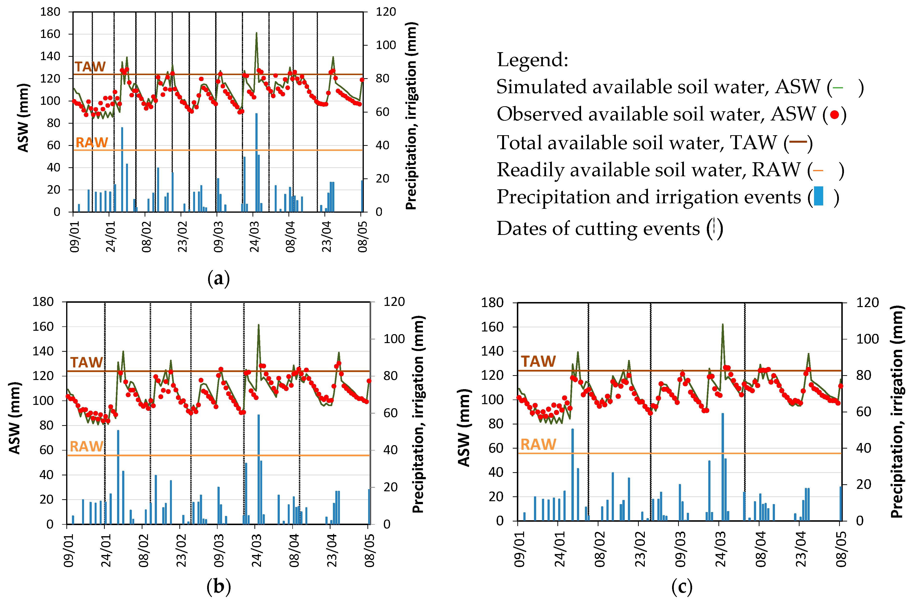
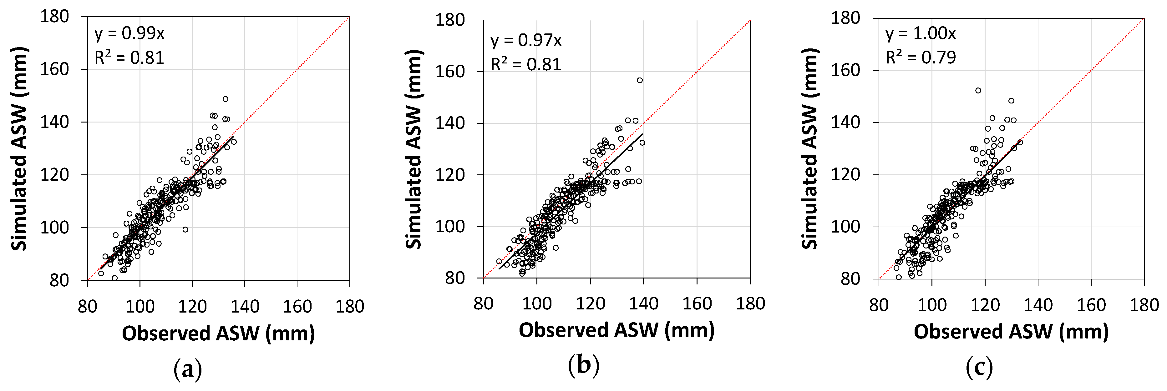
e curves for Tifton 85 to be obtained when managed with those three cutting intervals. Data of Summer and Autumn of 2016 were used for calibration and data for Spring 2015 and 2016, and Summer and Autumn of 2017 were used for validation. The procedure used led to quite small errors of estimation of the available soil water throughout both years, which allowed us to assume that the calibrated Kcb values were accurately estimated and may be considered as standard for the three cutting frequencies studied after adjustments with Equation (7). It is important to note that the estimation of the initial Kcb values from the crop cover and height has shown quite small differences to the calibrated values. Moreover, the Allen and Pereira [4] Equation (4) was revealed to be very accurate in estimating Kcb from h and fc provided that Kcb full is well estimated. The operational use of this Equation (4) is therefore recommended.
The Kcb curves consist of a series of Kcb curves relative to each cutting cycle, each one constructed with three linear segments. This approach follows the one proposed by the FAO56 guidelines [17] and differs from the commonly used single Kc curve. It was revealed to be accurate in describing crop transpiration and providing for the accuracy of soil water dynamics computed through the calibration and validation processes. However, for the case of very frequent cuttings (CGDD of 124 °C) there was no advantage over a single, averaged Kcb.
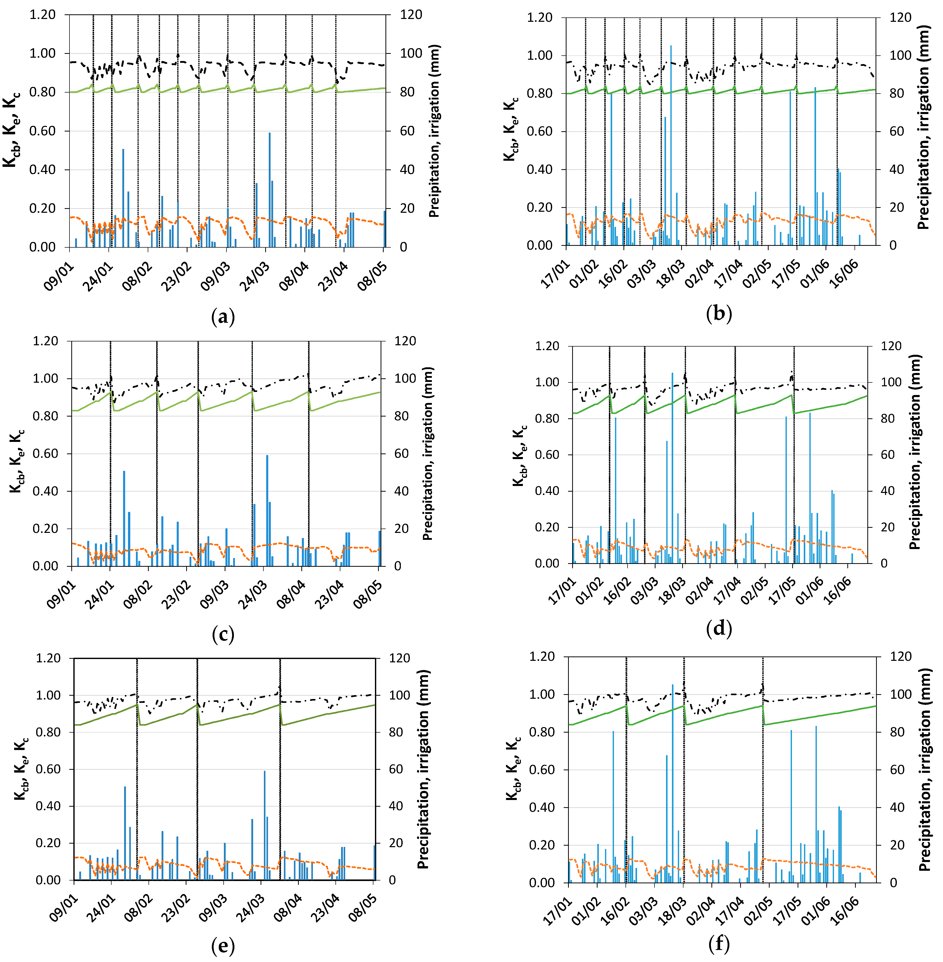
The Ke curve reflects the abundant and stormy rains that occurred in both years of field experiments, which made the soil evaporation layer wet most of the time. Thus, the Ke curve varied little throughout the periods under analysis. However, the soil water evaporation was mitigated due the organic mulch effect of the plant litter covering the ground, which reduced the energy available at the soil surface, thus reducing Ke and Es. Comparing Ke for the three cutting treatments, this resulted in a larger value for that with very frequent cuttings (CGDD of 124 °C) because the ground cover was smaller than for cuttings with large intervals, thus giving more time for the crop to grow and crop density to increase during each cutting cycle. Due to the nearly flat form of the Ke curve, the Kc curve and the sum of the Ke and Kcb curves do not reflect the aggregation of individual Kc curves relative to each cycle of cutting. Therefore, by contrast with the Kcb curves, a single Kc value is appropriate, however specific for each cutting treatment.
Results for the soil water balance are marked by the enormous amount of rain observed during these two years, likely due to the impacts of ENSO. Thus, the amount of runoff and, mainly, deep percolation exceeded crop ET. Thus, the option of irrigating to avoid any water stress was shown to be inappropriate despite not being prejudicial to the experiments. However, the large number of rainy days and the large amount of rain were likely associated with reduced solar radiation and temperature, which could have contributed to reduce transpiration and the Kcb values. However, the latter, as well as the Kc values, are larger than most of Kcb and Kc values reported in literature, which support the assumption that Kcb values may be considered standard and transferable to other locations after appropriate adjustments.
The soil evaporation fraction (Es/ETc) for all cases was small, near 13% in the case of frequent cuttings and about 9% when cuttings were less frequent. These values could slightly decrease if soil wettings were less frequent. These results indicate that beneficial consumptive water use by the crop is high, with the transpiration ratio near 90%. These results agree well with those reported in literature relative to well-managed grasslands, particularly tropical ones. This may indicate that the Tifton 85 bermudagrass has the potential to contribute to the sustainability of the Pampa biome in southern Brazil. Adopting a median cuttings frequency (CGDD of 248 °C) is likely the most favorable. However, more studies are required, mainly relative to herbage production and water productivity, which are expected to be undertaken based upon the field data used in the current study.
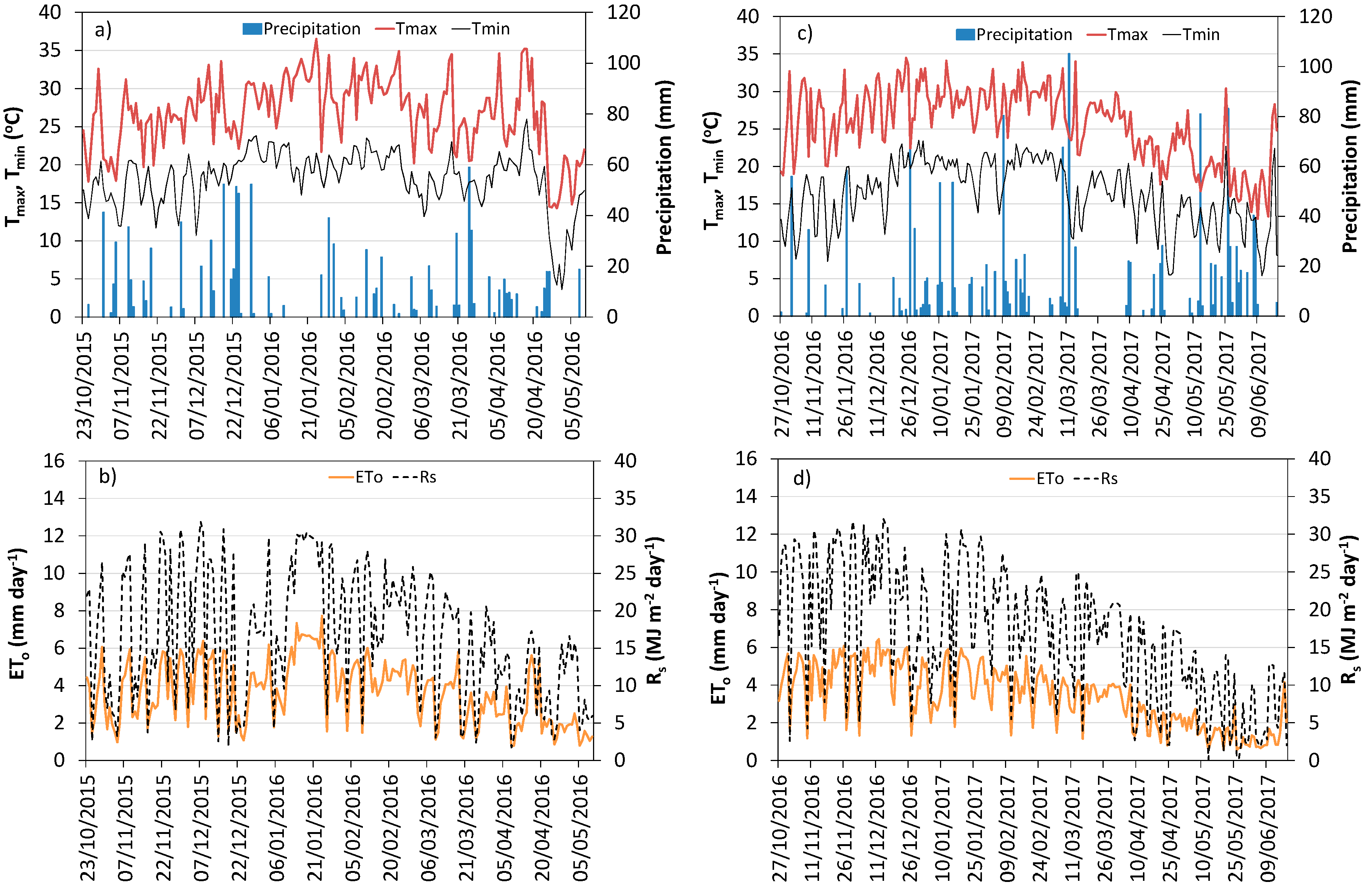
Author Contributions

Reimar Carlesso and Geraldo J. Rodrigues conceived and designed the experiments. Geraldo J. Rodrigues and Paula Severo O. performed the field experiments under the supervision of Reimar Carlesso. Geraldo J. Rodrigues and Mirta T. Petry handled the data with advice of Reimar Carlesso. Paula Paredes performed modelling with the advice of Luis S. Pereira, and writing was undertaken by Luis S. Pereira with the contributions of Mirta T. Petry and Paula Paredes.

Funding

This research was funded by CAPES/CNPq Post-Graduation Cooperative Program in Agricultural Engineering, Brazil, grant number 88881.030480/2013-01; Fundação para a Ciência e a Tecnologia, Portugal through the research unit LEAF-Linking Landscape, Environment, Agriculture and Food (UID/AGR/04129/2013) and the first author post-doc fellowship SFRH/BPD/102478/2014.

Conflicts of Interest

The authors declare no conflict of interest.

References

  1. Roesch, L.F.W.; Vieira, F.C.B.; Pereira, V.A.; Schünemann, A.L.; Teixeira, I.F.; Senna, A.J.T.; Stefenon, V.M. The Brazilian Pampa: A fragile biome. Diversity 2009, 1, 182–198. [Google Scholar] [CrossRef]
  2. Liu, K.; Sollenberger, L.E.; Newman, Y.C.; Vendramini, J.M.B.; Interrante, S.M.; White-Leech, R. Grazing management effects on productivity, nutritive value, and persistence of ‘Tifton 85’ Bermudagrass. Crop Sci. 2011, 51, 353–360. [Google Scholar] [CrossRef]
  3. Silva, V.J.; Pedreira, C.G.S.; Sollenberger, L.E.; Carvalho, M.S.S.; Tonato, F.; Basto, D.C. Seasonal herbage accumulation and nutritive value of irrigated ‘Tifton 85’, Jiggs, and Vaquero Bermudagrasses in response to harvest frequency. Crop Sci. 2015, 55, 1–9. [Google Scholar] [CrossRef]
  4. Allen, R.G.; Pereira, L.S. Estimating crop coefficients from fraction of ground cover and height. Irrig. Sci. 2009, 28, 17–34. [Google Scholar] [CrossRef]
  5. Monteith, J.L. Evaporation and environment. In The State and Movement of Water in Living Organisms, Proceedings of the 19th Symposium of the Society for Experimental Biology, Swansea, 1964; Cambridge University Press: Cambridge, UK, 1965; pp. 205–234. [Google Scholar]
  6. Priestley, C.H.B.; Taylor, R.J. On the assessment of surface heat flux and evaporation using large-scale parameters. Mon. Weather Rev. 1972, 100, 81–92. [Google Scholar] [CrossRef]
  7. Li, S.-G.; Lai, C.-T.; Lee, G.; Shimoda, S.; Yokoyama, T.; Higuchi, A.; Oikawa, T. Evapotranspiration from a wet temperate grassland and its sensitivity to microenvironmental variables. Hydrol. Process. 2005, 19, 517–532. [Google Scholar] [CrossRef]
  8. Ryu, Y.; Baldocchi, D.D.; Ma, S.; Hehn, T. Interannual variability of evapotranspiration and energy exchange over an annual grassland in California. J. Geophys. Res. 2008, 113, D09104. [Google Scholar] [CrossRef]
  9. Li, J.; Jiang, S.; Wang, B.; Jiang, W.-W.; Tang, Y.-H.; Du, M.-Y.; Gu, S. Evapotranspiration and its energy exchange in alpine meadow ecosystem on the Qinghai-Tibetan Plateau. J. Integr. Agric. 2013, 12, 1396–1401. [Google Scholar] [CrossRef]
  10. Savage, M.J.; Odhiambo, G.O.; Mengistu, M.G.; Everson, C.S.; Jarmain, C. Measurement of grassland evaporation using a surface-layer scintillometer. Water SA 2010, 36, 1–8. [Google Scholar] [CrossRef]
  11. Alfieri, J.G.; Xiao, X.; Niyogi, D.; Pielke, R.A., Sr.; Chen, F.; LeMone, M.A. Satellite-based modeling of transpiration from the grasslands in the Southern Great Plains, USA. Glob. Planet. Chang. 2009, 67, 78–86. [Google Scholar] [CrossRef]
  12. Courault, D.; Hadria, R.; Ruget, F.; Olioso, A.; Duchemin, B.; Hagolle, O.; Dedieu, G. Combined use of FORMOSAT-2 images with a crop model for biomass and water monitoring of permanent grassland in Mediterranean region. Hydrol. Earth Syst. Sci. 2010, 14, 1731–1744. [Google Scholar] [CrossRef] [Green Version]
  13. Krishnan, P.; Meyers, T.P.; Scott, R.L.; Kennedy, L.; Heuer, M. Energy exchange and evapotranspiration over two temperate semi-arid grasslands in North America. Agric. Forest Meteorol. 2012, 153, 31–44. [Google Scholar] [CrossRef]
  14. Kurc, S.A.; Small, E.E. Dynamics of evapotranspiration in semiarid grassland and shrubland ecosystems during the summer monsoon season, central New Mexico. Water Resour. Res. 2004, 40, W09305. [Google Scholar] [CrossRef]
  15. Moran, M.S.; Scott, R.L.; Keefer, T.O.; Emmerich, W.E.; Hernandez, M.; Nearing, G.S.; Paige, G.B.; Cosh, M.H.; O’Neill, P.E. Partitioning evapotranspiration in semiarid grassland and shrubland ecosystems using time series of soil surface temperature. Agric. Forest Meteorol. 2009, 149, 59–72. [Google Scholar] [CrossRef]
  16. Zha, T.; Barr, A.G.; van der Kamp, G.; Black, T.A.; McCaughey, J.H.; Flanagan, L.B. Interannual variation of evapotranspiration from forest and grassland ecosystems in western Canada in relation to drought. Agric. For. Meteorol. 2010, 150, 1476–1484. [Google Scholar] [CrossRef]
  17. Allen, R.G.; Pereira, L.S.; Raes, D.; Smith, M. Crop Evapotranspiration—Guidelines for Computing Crop Water Requirements; FAO Irrigation and Drainage Paper 56; FAO: Rome, Italy, 1998; p. 300. [Google Scholar]
  18. Pequeno, D.N.L.; Pedreira, C.G.S.; Sollenberger, L.E.; de Faria, A.F.G.; Silva, L.S. Forage accumulation and nutritive value of brachiariagrasses and Tifton 85 Bermudagrass as affected by harvest frequency and irrigation. Agron. J. 2015, 107, 1741–1749. [Google Scholar] [CrossRef]
  19. Thornthwaite, C.W. An approach toward a rational classification of climate. Geogr. Rev. 1948, 38, 55–94. [Google Scholar] [CrossRef]
  20. Zhao, Y.; Peth, S.; Horn, R.; Krümmelbein, J.; Ketzer, B.; Gao, Y.; Doerner, J.; Bernhofer, C.; Peng, X. Modeling grazing effects on coupled water and heat fluxes in Inner Mongolia grassland. Soil Till. Res. 2010, 109, 75–86. [Google Scholar] [CrossRef]
  21. Qassim, A.; Dunin, F.; Bethune, M. Water balance of centre pivot irrigated pasture in northern Victoria, Australia. Agric. Water Manag. 2008, 95, 566–574. [Google Scholar] [CrossRef]
  22. Sumner, D.M.; Jacobs, J.M. Utility of Penman–Monteith, Priestley–Taylor, reference evapotranspiration, and pan evaporation methods to estimate pasture evapotranspiration. J. Hydrol. 2005, 308, 81–104. [Google Scholar] [CrossRef]
  23. Wherley, B.; Dukes, M.D.; Cathey, S.; Miller, G.; Sinclair, T. Consumptive water use and crop coefficients for warm-season turfgrass species in the Southeastern United States. Agric. Water Manag. 2015, 156, 10–18. [Google Scholar] [CrossRef]
  24. Neal, J.S.; Fulkerson, W.J.; Hacker, R.B. Differences in water use efficiency among annual forages used by the dairy industry under optimum and deficit irrigation. Agric. Water Manag. 2011, 98, 759–774. [Google Scholar] [CrossRef]
  25. Zhang, F.; Zhou, G.; Wang, Y.; Yang, F.; Nilsson, C. Evapotranspiration and crop coefficient for a temperate desert steppe ecosystem using eddy covariance in Inner Mongolia, China. Hydrol. Process. 2012, 26, 379–386. [Google Scholar] [CrossRef]
  26. Pronger, J.; Campbell, D.I.; Clearwater, M.J.; Rutledge, S.; Wall, A.M.; Schipper, L.A. Low spatial and inter-annual variability of evaporation from a year-round intensively grazed temperate pasture system. Agric. Ecosyst. Environ. 2016, 232, 46–58. [Google Scholar] [CrossRef]
  27. Cancela, J.J.; Cuesta, T.S.; Neira, X.X.; Pereira, L.S. Modelling for improved irrigation water management in a temperate region of Northern Spain. Biosyst. Eng. 2006, 94, 151–163. [Google Scholar] [CrossRef]
  28. Pereira, L.S.; Teodoro, P.R.; Rodrigues, P.N.; Teixeira, J.L. Irrigation scheduling simulation: The model ISAREG. In Tools for Drought Mitigation in Mediterranean Regions; Rossi, G., Cancelliere, A., Pereira, L.S., Oweis, T., Shatanawi, M., Zairi, A., Eds.; Kluwer Academic Press: Dordrecht, The Netherlands, 2003; pp. 161–180. [Google Scholar]
  29. Pôças, I.; Cunha, M.; Pereira, L.S.; Allen, R.G. Using remote sensing energy balance and evapotranspiration to characterize montane landscape vegetation with focus on grass and pasture lands. Int. J. Appl. Earth Observ. 2013, 21, 159–172. [Google Scholar] [CrossRef]
  30. Pakparvar, M.; Cornelis, W.; Pereira, L.S.; Gabriels, D.; Hafeez, M.; Hosseinimarandi, H.; Edraki, M.; Kowsar, S.A. Remote sensing estimation of actual evapotranspiration and crop coefficients for a multiple land use arid landscape of southern Iran with limited available data. J. Hydroinform. 2014, 16, 1441–1460. [Google Scholar] [CrossRef]
  31. Jia, X.; Dukes, M.D.; Jacobs, J.M. Bahiagrass crop coefficients from eddy correlation measurements in central Florida. Irrig. Sci. 2009, 28, 5–15. [Google Scholar] [CrossRef]
  32. Allen, R.G.; Pereira, L.S.; Smith, M.; Raes, D.; Wright, J.L. FAO-56 Dual crop coefficient method for estimating evaporation from soil and application extensions. J. Irrig. Drain. Eng. 2005, 131, 2–13. [Google Scholar] [CrossRef]
  33. Greenwood, K.L.; Lawson, A.R.; Kelly, K.B. The water balance of irrigated forages in northern Victoria, Australia. Agric. Water Manag. 2009, 96, 847–858. [Google Scholar] [CrossRef]
  34. Wu, Y.; Liu, T.; Paredes, P.; Duan, L.; Wang, H.; Wang, T.; Pereira, L.S. Ecohydrology of groundwater-dependent grasslands of the semi-arid Horqin sandy land of inner Mongolia focusing on evapotranspiration partition. Ecohydrology 2016, 9, 1052–1067. [Google Scholar] [CrossRef]
  35. Rosa, R.D.; Paredes, P.; Rodrigues, G.C.; Alves, I.; Fernando, R.M.; Pereira, L.S.; Allen, R.G. Implementing the dual crop coefficient approach in interactive software. 1. Background and computational strategy. Agric. Water Manag. 2012, 103, 8–24. [Google Scholar] [CrossRef]
  36. Krauß, M.; Kraatz, S.; Drastig, K.; Prochnow, A. The influence of dairy management strategies on water productivity of milk production. Agric. Water Manag. 2015, 147, 175–186. [Google Scholar] [CrossRef]
  37. Paredes, P.; Rodrigues, G.C.; Alves, I.; Pereira, L.S. Partitioning evapotranspiration, yield prediction and economic returns of maize under various irrigation management strategies. Agric. Water Manag. 2014, 135, 27–39, Corrigendum in Agric. Water Manag. 2014, 141, 84. [Google Scholar] [CrossRef]
  38. Zhao, N.; Liu, Y.; Cai, J.; Paredes, P.; Rosa, R.D.; Pereira, L.S. Dual crop coefficient modelling applied to the winter wheat–summer maize crop sequence in North China Plain: Basal crop coefficients and soil evaporation component. Agric. Water Manag. 2013, 117, 93–105. [Google Scholar] [CrossRef]
  39. Pereira, L.S.; Paredes, P.; Rodrigues, G.C.; Neves, M. Modeling barley water use and evapotranspiration partitioning in two contrasting rainfall years. Assessing SIMDualKc and AquaCrop models. Agric. Water Manag. 2015, 159, 239–254. [Google Scholar] [CrossRef]
  40. Wei, Z.; Paredes, P.; Liu, Y.; Chi, W.-W.; Pereira, L.S. Modelling transpiration, soil evaporation and yield prediction of soybean in North China Plain. Agric. Water Manag. 2015, 147, 43–53. [Google Scholar] [CrossRef]
  41. Paço, T.A.; Ferreira, M.I.; Rosa, R.D.; Paredes, P.; Rodrigues, G.C.; Conceição, N.; Pacheco, C.A.; Pereira, L.S. The dual crop coefficient approach using a density factor to simulate the evapotranspiration of a peach orchard: SIMDualKc model vs. eddy covariance measurements. Irrig. Sci. 2012, 30, 115–126. [Google Scholar] [CrossRef]
  42. Paço, T.A.; Pôças, I.; Cunha, M.; Silvestre, J.C.; Santos, F.L.; Paredes, P.; Pereira, L.S. Evapotranspiration and crop coefficients for a super intensive olive orchard. An application of SIMDualKc and METRIC models using ground and satellite observations. J. Hydrol. 2014, 519, 2067–2080. [Google Scholar] [CrossRef]
  43. Shuttleworth, W.J.; Wallace, J.S. Evaporation from sparse crops-an energy combination theory. Q. J. R. Meteorol. Soc. 1985, 111, 839–855. [Google Scholar] [CrossRef]
  44. Hu, Z.; Yu, G.; Zhou, Y.; Sun, X.; Li, Y.; Shi, P.; Wang, Y.; Song, X.; Zheng, Z.; Zhang, L.; Li, S. Partitioning of evapotranspiration and its controls in four grassland ecosystems: Application of a two-source model. Agric. For. Meteorol. 2009, 149, 1410–1420. [Google Scholar] [CrossRef]
  45. Kochendorfer, J.P.; Ramírez, J.A. Modeling the monthly mean soil-water balance with a statistical-dynamical ecohydrology model as coupled to a two-component canopy model. Hydrol. Earth Syst. Sci. 2010, 14, 2099–2120. [Google Scholar] [CrossRef] [Green Version]
  46. Huang, X.; Hao, Y.; Wang, Y.; Cui, X.; Mo, X.; Zhou, X. Partitioning of evapotranspiration and its relation to carbon dioxide fluxes in Inner Mongolia steppe. J. Arid Environ. 2010, 74, 1616–1623. [Google Scholar] [CrossRef]
  47. Wang, P.; Yamanaka, T. Application of a two-source model for partitioning evapotranspiration and assessing its controls in temperate grasslands in central Japan. Ecohydrology 2014, 7, 345–353. [Google Scholar] [CrossRef]
  48. Graham, S.L.; Kochendorfer, J.; McMillan, A.M.S.; Duncan, M.J.; Srinivasan, M.S.; Hertzog, G. Effects of agricultural management on measurements, prediction, and partitioning of evapotranspiration in irrigated grasslands. Agric. Water Manag. 2016, 177, 340–347. [Google Scholar] [CrossRef]
  49. Ferretti, D.F.; Pendall, E.; Morgan, J.A.; Nelson, J.A.; LeCain, D.; Mosier, A.R. Partitioning evapotranspiration fluxes from a Colorado grassland using stable isotopes: Seasonal variations and ecosystem implications of elevated atmospheric CO2. Plant Soil 2003, 254, 291–303. [Google Scholar] [CrossRef]
  50. Hu, Z.; Wen, X.; Sun, X.; Li, L.; Yu, G.; Lee, X.; Li, S. Partitioning of evapotranspiration through oxygen isotopic measurements of water pools and fluxes in a temperate grassland. J. Geophys. Res. Biogeosci. 2014, 119, 358–371. [Google Scholar] [CrossRef]
  51. Kottek, M.; Grieser, J.; Beck, C.; Rudolf, B.; Rubel, F. World Map of the Köppen-Geiger climate classification updated. Meteorol. Z. 2006, 15, 259–263. [Google Scholar] [CrossRef]
  52. Ritchie, J.T. Model for predicting evaporation from a row crop with incomplete cover. Water Resour. Res. 1972, 8, 1204–1213. [Google Scholar] [CrossRef]
  53. Liu, Y.; Pereira, L.S.; Fernando, R.M. Fluxes through the bottom boundary of the root zone in silty soils: Parametric approaches to estimate groundwater contribution and percolation. Agric. Water Manag. 2006, 84, 27–40. [Google Scholar] [CrossRef]
  54. Hydrologic Soil-Cover Complexes. In National Engineering Handbook Hydrology; USDA-NRCS: Washington, DC, USA, 2004. Available online: https://www.wcc.nrcs.usda.gov/ftpref/wntsc/H&H/NEHhydrology/ch9.pdf (accessed on 14 March 2018).
  55. Liu, K.; Sollenberger, L.E.; Silveira, M.L.; Newman, Y.C.; Vendramini, J.M.B. Grazing intensity and nitrogen fertilization affect litter responses in ‘Tifton 85’ Bermudagrass pastures: I. Mass, deposition rate, and chemical composition. Agron. J. 2011, 103, 156–162. [Google Scholar] [CrossRef]
  56. Martins, J.D.; Rodrigues, G.C.; Paredes, P.; Carlesso, R.; Oliveira, Z.B.; Knies, A.E.; Petry, M.T.; Pereira, L.S. Dual crop coefficients for maize in southern Brazil: Model testing for sprinkler and drip irrigation and mulched soil. Biosyst. Eng. 2013, 115, 291–310. [Google Scholar] [CrossRef]
  57. Fandiño, M.; Olmedo, J.L.; Martínez, E.M.; Valladares, J.; Paredes, P.; Rey, B.J.; Mota, M.; Cancela, J.J.; Pereira, L.S. Assessing and modelling water use and the partition of evapotranspiration of irrigated hop (Humulus lupulus), and relations of transpiration with hops yield and alpha-acids. Ind. Crops Prod. 2015, 77, 204–217. [Google Scholar] [CrossRef]
  58. Moriasi, D.N.; Arnold, J.G.; Van Liew, M.W.; Bingner, R.L.; Harmel, R.D.; Veith, T.L. Model evaluation guidelines for systematic quantification of accuracy in watershed simulations. Trans. ASABE 2007, 50, 885–900. [Google Scholar] [CrossRef]
  59. Nash, J.E.; Sutcliffe, J.V. River flow forecasting through conceptual models: Part 1. A discussion of principles. J. Hydrol. 1970, 10, 282–290. [Google Scholar] [CrossRef]
  60. Schlesinger, W.H.; Jasechko, S. Transpiration in the global water cycle. Agric. For. Meteorol. 2014, 189–190, 115–117. [Google Scholar] [CrossRef]
  61. Pereira, L.S.; Cordery, I.; Iacovides, I. Improved indicators of water use performance and productivity for sustainable water conservation and saving. Agric. Water Manag. 2012, 108, 39–51. [Google Scholar] [CrossRef]
Figure 1. Daily weather data during the crop seasons of 2015/16 and 2016/17: (a,c) maximum ( Water 10 00558 i001) and minimum ( Water 10 00558 i002) temperatures, and rainfall ( Water 10 00558 i003); (b,d) solar radiation ( Water 10 00558 i004) and reference evapotranspiration ( Water 10 00558 i005).
Water 10 00558 g001
Figure 2. Simulated vs. observed available soil water during the Summer-Autumn of 2016 relative to the calibration of SIMDualKc model for treatments of CGDD of: (a) 124 °C, (b) 248 °C and (c) 372 °C.
Water 10 00558 g002
Figure 3. Simulated vs. observed available soil water (ASW) relative to the validation of SIMDualKc model for treatments of CGDD of: (a) 124 °C, (b) 248 °C and (c) 372 °C.
Water 10 00558 g003
Figure 4. Basal crop coefficient (Kcb, Water 10 00558 i006), soil evaporation coefficient (Ke, Water 10 00558 i007) and average crop coefficient (Kc, Water 10 00558 i008) curves of Tifton 85 bermudagrass and all cutting treatments with CGDD of 124 °C (a,b), 248 °C (c,d) and 372 °C (e,f) relative to the Summer–Autumn periods of 2016 (a,c,e) and 2017 (b,d,f).
Water 10 00558 g004
Table 1. Soil physical characteristics of the experimental field.
Depth (cm)Bulk Density (g cm−3)Total Porosity (%)Field Capacity (FC) (cm3·cm−3)Wilting Point (WP) (cm3·cm−3)Clay %Silt %Sand %
0–51.4941.30.3640.089183646
5–101.5638.60.3370.085183646
10–151.4743.20.2980.081203545
15–301.5142.00.3750.087203743
30–501.5043.00.3080.092243541
Table 2. Cuttings dates of the various treatments having different cumulative growing degree days (CGDD) intervals between cuttings.
EventsCutting TreatmentsDates
CGDD of 124 °CCGDD of 248 °CCGDD of 372 °CSeason of 2015/16Season of 2016/17
Spring (t0) 23 October 201527 October 2016
Scheduled cuttings1st 4 November 201510 November 2016
2nd1st 15 November 201522 November 2016
3rd 1st27 November 20152 December 2016
4th2nd 8 December 201512 December 2016
5th 17 December 201522 December 2016
6th3rd2nd28 December 201529 December 2016
Summer-Autumn (t0) 9 January 201617 January 2017
Scheduled cuttings1st 16 January 201627 January 2017
2nd1st 24 January 20165 February 2017
3rd 1st3 February 201615 February 2017
4th2nd 10 February 201623 February 2017
5th 18 February 20166 March 2017
6th3rd2nd26 February 201619 March 2017
7th 8 March 20162 April 2017
8th4th 18 March 201613 April 2017
9th 3rd30 March 201627 April 2017
10th5th 9 April 201615 May 2017
11th 18 April 20165 May 2017
12th6th4th08 May 201626 June 2017
Table 3. Time intervals between cuttings for all treatments.
Cutting TreatmentsMinimum Intervals (Days) Maximum Intervals (Days)
2015–20162016–20172015–20162016–2017
CGDD of 124 °C9102021
CGDD of 248 °C20172942
CGDD of 372 °C31273960
Table 4. Average of observed canopy height (h, m) and fraction of ground cover (fc, dimensionless) relative to treatments with various intervals between cuttings defined by observed CGDD.
Variables and TreatmentsGrass Development Stages
InitialEnd of Rapid GrowthBefore Cutting
Canopy height (h, m)hinihgrohcut
CGDD of 124 °C0.150.180.19
CGDD of 248 °C0.150.220.23
CGDD of 372 °C0.150.270.30
Fraction of ground cover (fc, dimensionless)fc inifc grofc cut
CGDD of 124 °C0.810.850.90
CGDD of 248 °C0.810.880.92
CGDD of 372 °C0.850.900.93
Table 5. Initial and calibrated parameters of SIMDualKc relative to the three treatments of Tifton 85 bermudagrass having different frequency of cuttings.
ParametersSymbolsInitial ValuesCalibrated Values
CGDD of 124 °CCGDD of 248 °CCGDD of 372 °CCGDD of 124 °CCGDD of 248 °CCGDD of 372 °C
Basal crop coefficientsKcb ini0.770.820.840.800.830.84
Kcb gro0.800.870.890.820.880.90
Kcb cut0.840.900.910.840.930.94
Depletion fractionp0.550.55
Soil evaporationZe (m)0.150.15
REW (mm)1010
TEW (mm)3744
Deep percolationaD335325
bD−0.017−0.005
RunoffCN7074
Ze = Depth of the soil evaporation layer; REW = Readily evaporable water; TEW =Total evaporable water; aD and bD = parameters of the deep percolation equation [53]; CN = Curve number
Table 6. Goodness-of-fit indicators relative to both the calibration and validation of all treatments.
Cuttings IntervalPeriodGoodness-of-Fit Indicators
b0R2RMSE (mm)NRMSE (%)ARE (%)PBIAS (%)EF
Calibration
CGDD of 124 °CSummer–Autumn 20161.010.815.24.94.0−0.90.76
CGDD of 248 °CSummer–Autumn 20161.000.874.24.03.2−0.30.86
CGDD of 372 °CSummer–Autumn 20161.010.864.84.53.6−0.70.77
Validation
CGDD of 124 °CSpring 20151.000.835.24.83.40.20.79
Spring 20160.980.715.35.23.41.60.61
Summer–Autumn 20170.990.806.05.44.50.80.75
CGDD of 248 °CSpring 20150.970.766.75.95.23.00.47
Spring 20160.970.855.04.94.02.70.71
Summer–Autumn 20170.970.787.26.45.02.70.62
CGDD of 372 °CSpring 20151.010.757.26.74.0−1.30.52
Spring 20160.980.676.56.34.72.10.42
Summer–Autumn 20171.000.825.85.44.40.60.72
RMSE = Root mean square error; NRMSE = Normalized RMSE; ARE = Average relative error; PBIAS = Percent bias of estimation; EF = Modelling efficiency
Table 7. Goodness-of-fit indicators for the treatment relative to frequent cuttings with CGDD of 124 °C when adopting a single Kcb = 0.80.
PeriodGoodness-of-Fit Indicators
b0R2RMSE (mm)NRMSE (%)ARE (%)PBIAS (%)EF
CalibrationSummer–Autumn 20161.000.795.55.24.2−0.40.73
ValidationSpring 20150.990.854.84.43.41.10.82
Spring 20160.980.697.06.84.32.30.43
Summer–Autumn 20170.990.805.95.44.41.00.75
Table 8. Standard crop coefficients for Tifton 85 bermudagrass as dependent on the frequency of cuttings.
Treatment
CGDD of 124 °CCGDD of 248 °CCGDD of 372 °C
Kcb ini0.830.860.87
Kcb gro0.850.910.93
Kcb cut0.870.960.97
Kc0.960.991.00
Table 9. Soil water balance terms (mm) for all cutting treatments and all observation periods.
Cuttings TreatmentsPeriodPIΔSWRODPETcEsTc
CGDD of 124 °CSpring, 20154842275822123432202
Summer–Autumn, 2016529108−31720641153358
Spring, 2016320123−201613427337236
Summer–Autumn, 20171076612819255641755363
CGDD of 248 °CSpring, 201548422215822924023217
Summer–Autumn, 2016529108−41619642137384
Spring, 2016320123−241611928425259
Summer–Autumn, 20171076612619254742839389
CGDD of 372 °CSpring, 201548422105821724122219
Summer–Autumn, 2016529108−51519242536389
Spring, 2016320123−201612528225257
Summer–Autumn, 20171076611819252943439395
P = precipitation, I = irrigation, ΔSW = variation in stored soil water, DP= deep percolation, RO = runoff; Es = soil evaporation, Tc = crop transpiration, ETc = crop evapotranspiration.
Table 10. Crop evapotranspiration (ETc, mm) and evaporation and transpiration ratios (Es/ETc and Tc/ETc, %) for all cutting treatments and observation periods.
Cutting TreatmentsPeriodETc (mm)Es/ETc (%)Tc/ETc (%)
CGDD of 124 °CSpring, 20152341486
Summer–Autumn, 20164111387
Spring, 20162731486
Summer–Autumn, 20174171387
CGDD of 248 °CSpring, 20152401090
Summer–Autumn, 2016421991
Spring, 2016284991
Summer–Autumn, 2017428991
CGDD of 372 °CSpring, 2015241991
Summer–Autumn, 2016425892
Spring, 2016282991
Summer–Autumn, 2017434991

