Design Flood Estimation Methods for Cascade Reservoirs Based on Copulas


State Key Laboratory of Water Resources and Hydropower Engineering Science, Hubei Provincial Collaborative Innovative Center for Water Resources Security, Wuhan University, Wuhan 430072, China
*
Author to whom correspondence should be addressed.
Water 2018, 10(5), 560; https://doi.org/10.3390/w10050560
Submission received: 20 March 2018
/
Revised: 16 April 2018
/
Accepted: 23 April 2018
/
Published: 26 April 2018
(This article belongs to the Special Issue Advances in Multivariate Analysis of Environmental Phenomena: Celebrating the 15th Anniversary of Copulas in Hydrology)
Abstract
:Reservoirs operation alters the natural flow regime at downstream site and thus has a great impact on the design flood values. The general framework of flood regional composition and Equivalent Frequency Regional Composition (EFRC) method are currently used to calculate design floods at downstream site while considering the impact of the upstream reservoirs. However, this EFRC method deems perfect correlation between peak floods that occurred at one sub-basin and downstream site, which implicitly assumes that the rainfall and the land surface process are uniformly distributed for various sub-basins. In this study, the Conditional Expectation Regional Composition (CERC) method and Most Likely Regional Composition (MLRC) method based on copula function are proposed and developed under the flood regional composition framework. The proposed methods (i.e., CERC and MLRC) are tested and compared with the EFRC method in the Shuibuya-Geheyan-Gaobazhou cascade reservoirs located at Qingjiang River basin, a tributary of Yangtze River in China. Design flood values of the Gaobazhou reservoir site are estimated under the impact of upstream cascade reservoirs, respectively. Results show that design peak discharges at the Gaobazhou dam site have been significantly reduced due to the impact of upstream reservoir regulation. The EFRC method, not taking the actual dependence of floods occurred at various sub-basins into account; as a consequence, it yields an under-or overestimation of the risk that is associated with a given event in hydrological design. The proposed methods with stronger statistical basis can better capture the actual spatial correlation of flood events occurred at various sub-basins, and the estimated design flood values are more reasonable than the currently used EFRC method. The MLRC method is recommended for design flood estimation in the cascade reservoirs since its composition is unique and easy to implement.
1. Introduction
Design flood estimation is often required by engineers, hydrologists, and agriculturalists for the design of hydraulic structures, such as dams, bridges, or culverts. The choice of design flood values has a great impact not only on the investment and benefit of the project, but also on the safety of the infrastructures [1,2,3,4].
When sufficiently long observed flow records (the annual maximum peak discharge or flood volume series) at the interest site are available, the design flood values are generally estimated from flood frequency analysis. The main modeling problem in flood frequency analysis is the selection of a probability distribution for flood magnitudes coupled with the choice of parameter estimation procedures [5]. Probability distributions provide the essential basic formulae to model a flood quantile in terms of its exceedance probability. Once a distribution is selected, the next step is to estimate its parameters. Different probability distributions are proposed and used depending on, among others, the climatic and the geographical characteristics of the study region. In the United States, the log-Pearson type III (LP3) distribution is recommended as the candidate distribution for defining the annual maximum flood series, and the method of moments is used to determine the statistical parameters [6]. The Pearson type III (P3) distribution and curve fitting procedure are recommended by the Ministry of Water Resources of China as a standard procedure for flood frequency analysis [3]. The Generalized Logistic (GL) distribution is found to be more suitable for United Kingdom (UK) flood data [7]. The L-moments approach is preferred for parameter estimation because of its robust properties in the presence of usually small or large values (outliers) and is recommended by many authors. However, this conventional flood frequency analysis method is mainly concentrated on the analysis of annual maximum flood series in the natural condition.
In recent decades, many reservoirs have been built in river basins for flood prevention, hydropower generation, and water supply to meet the need of world population growth and rapid social economy development [2,8,9]. Reservoirs cause important changes in the river regime downstream by altering the spatial and temporal distribution of the river flow [10]. During the flood season, a reservoir stores flood runoff and it then releases downstream to the channel over a longer period of time. This operation reduces the peak discharge of inflow, resulting in lower water-surface elevation and less damage [11]. In this case, the observed flood records at the downstream site are no longer natural due to the operation of upstream reservoirs. Correspondingly, the discharge magnitude-frequency curve (or design flood values) in the natural condition can not represent the real flood regime and characteristic under the long-term condition [12,13]. Therefore, the operation rules of the upstream reservoirs should be involved in the estimation of the downstream design floods. Unfortunately, few research works considering this impact could be found in the reference literature.
Under the influence of upstream reservoirs, the inflow contributing watersheds to downstream site consists of various sub-basins (including reservoir sites and interval basins) and the inflow of reservoirs has been transformed into outflow by man-made operation rules. This situation makes the determination of design flood values at the downstream site very complex and difficult. The impact of reservoirs operation on the downstream design floods depends on (1) the characteristics of the reservoirs, e.g., capacity and operation rules, for that the reservoir capacity limits the amount of runoff that can be collected and held for release at a non-damaging rate, and the operation rules determine the manner of release; (2) the proportion of reservoir inflow to flood that occurred at the downstream site. The proportion of reservoir site governs the amount of runoff that the reservoir can control, since a reservoir will store only inflow from the upstream area [11]. In general, the bigger the proportion of upstream reservoir basin, the larger the impact of reservoir on design floods at downstream.
Conventionally, the general framework of flood regional composition is used to determine the design flood values at downstream site of reservoirs. This general framework includes two steps [13]. First, it is assumed that there are no reservoirs exist and various sub-basins are in the natural condition. A design flood event with probability p is selected from the natural flood magnitude-frequency curve at downstream site. It requires searching for appropriate combinations of floods that occurred at various sub-basins in the natural condition. The corresponding natural design flood hydrograph at various sub-basins are derived by using the same flood amplification ratio of their respective typical flood hydrograph [14,15]. Then, the design flood at the downstream site under the influence of upstream reservoir can be obtained through flood routing by incorporating operation rules. The influenced design flood is assigned the same probability p as that of the natural condition.
When the characteristics of the reservoir are determined, the most important issue is to find an appropriate combination of floods that occurred at various sub-basins [16]. It can be easily seen that the number of possible flood regional combination is countless. But, these infinite combinations are generally not equivalent from a practical point of view. Indeed, different combination can result in different design flood values at downstream site under the influence of upstream reservoirs. Moreover, the combinations differ also in terms of their probability of occurrence, which is measured by the joint probability density function. Therefore, how to select appropriate combinations (i.e., flood regional composition method) is extremely important. In practice, several combinations, such as the most likely, the worst, and the best combinations, should be selected to evaluate the impact of upstream reservoirs on design flood at downstream site [17].
The Equivalent Frequency Regional Composition (EFRC) method has been recommended by the Ministry of Water Resources of China [3]. However, the EFRC method deems perfect correlation between peak floods that occurred at one sub-basin and downstream site, which implicitly assumes that the rainfall and the hydrologic surface process are uniformly distributed for all of the sub-basins. In real case, there are different correlations (or dependence) between the sub-basins due to spatial and temporal variation of rainfall and land surface process. It therefore often makes the design flood fails to meet the flood prevention standard at the downstream site since the resulting design flood value is neither the most likely nor the worst composition. Furthermore, the currently used EFRC method can only be applied step by step to complex cascade reservoirs, which is not only difficult to implement, but is also subjective to some degree [3,13]. Flood regional composition is the stochastic combinations of flood variables (peak or volume) at different sub-basins, and the scientific way to analyse this problem is based on the joint distribution of these related variables. In recent years, much progress has been made in the method of joint probability distribution simulation, including the successful application of copula functions in hydrology. Copulas have been introduced in hydrology by De Michele and Salvadori in 2003 [18]. The first multivariate frequency analysis and return period calculation, multivariate design, multivariate hazard scenarios, and corresponding failure probabilities were given by Salvadori and De Michele [19], Salvadori et al. [20,21]. There are manifold advantages in using copulas to model joint distributions: they give (a) flexibility in choosing arbitrary marginal distribution and structure of dependence; (b) easier extension to more than two variables; and, (c) separate analysis of marginal distribution and dependence structure [12,18,19,20,21,22,23,24,25,26,27,28,29,30,31,32,33]. Therefore, the copula function can offer an effective tool to search for appropriate flood regional compositions.
This study aims to improve the flood regional composition method for design flood estimation of cascade reservoirs. The structure of the paper is as follows. Section 2 outlines the general framework of the flood regional composition and briefly introduces the currently used EFRC method. Section 3 presents the methodology of two flood regional composition methods, i.e., the Conditional Expectation Regional Composition (CERC) method and the Most Likely Regional Composition (MLRC) method based on the copula function. Section 4 reports a case study of the Shuibuya-Geheyan-Gaobazhou cascade reservoirs that were located at the Qingjiang River, which is a tributary of Yangtze River in China using the two proposed methods and compared with the EFRC method. Section 5 contains some discussions. Section 6 summarizes the conclusions.
2. Flood Regional Composition
2.1. General Framework of Flood Regional Composition
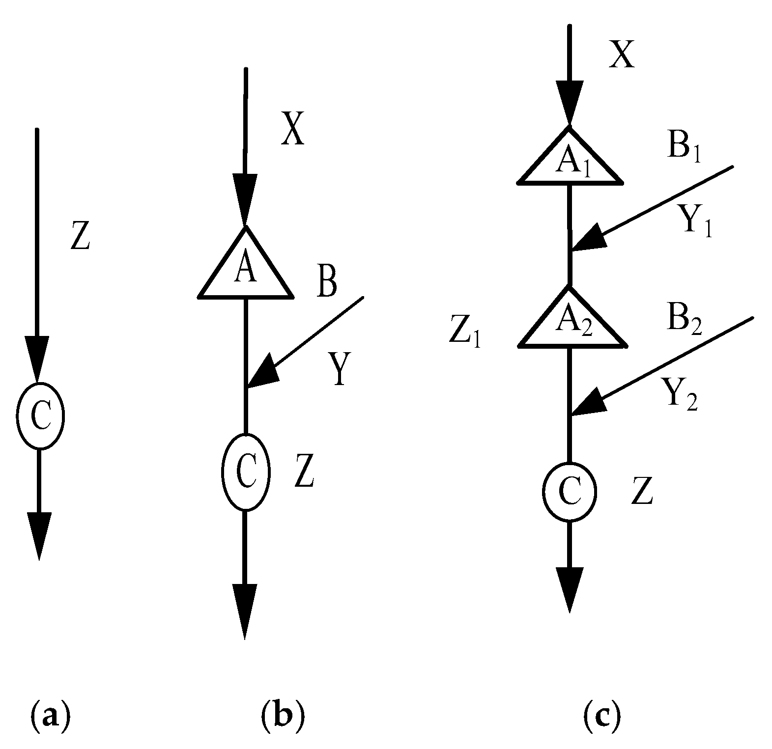
A sketch diagram of natural rivers and reservoir systems is shown in Figure 1, in which C denotes downstream site and zp represents flood characteristic variables (flood peak or volume) of site C with the corresponding design probability p. In the case of Figure 1a, when adequate observed flow data, i.e., the annual maximum peak discharge or flood volume series at site C is available, the general methodology of estimating design flood for site C is to derive the fitted theoretical distribution (e.g., P3 or LP3), representing the probability of z being exceeded based on the univariate distribution [3,6]). This conventional method is based on the assumption that the annual maximum flood series are statistically independent and identically distributed (i.i.d.) [5].
Once the reservoir A has been constructed at upstream of site C, as shown in Figure 1b, the operation rules of the upstream reservoir A should be involved in estimating design flood at site C. The inflow contributing watershed area to site C is divided into two parts, one is up to the reservoir A, and the other is the interval basin B between reservoir A and site C. In this condition, the flood regional composition framework is used to determine the design flood values at downstream site C under the influence of upstream reservoir A.
Flood regional composition is studied in the natural condition, which aims to search for an appropriate combination of corresponding floods that occurred at reservoir A and interval basin B by decomposition of floods occurred at downstream site C [16]. It represents the spatial relation between floods that occurred at various sub-basins and downstream site C in the natural condition. For a large or medium-size reservoir, the flood routing operation is usually controlled by the flood volume, so the regional combination is usually referred to flood volume for convenience.
Let random variables X, Y, and Z represent natural flood volume of the reservoir A, interval basin B, and downstream site C, respectively, with the corresponding values x, y, and z. According to the principle of water balance (the flood volume at site C is the summation of flood volume at reservoir A and interval basin B in the natural condition), all of the combinations (x, y) should be subjected to the following equation [11]:
Once the combination (x, y) is determined using the flood regional composition method, the following procedure is used to calculate the design flood at site C: (1) Selecting a typical inflow hydrograph at the reservoir A and interval basin B from the observed inflow records, respectively; (2) calculating the corresponding design flood hydrograph at the reservoir A and the interval basin B by using the same flood amplification ratio of their respective typical flood hydrograph [15,33]; (3) routing these two corresponding design flood hydrographs through the reservoir A according to its operation rules; and, (4) obtaining the flood hydrograph and design flood value at site C under the influence of reservoir A operation by the summation of these two routed flow hydrographs, which is assigned the same probability with that of the natural condition [3,11].
Cascade reservoirs consisting of an upper and a lower reservoir is the most common and representative circumstance. Multi-reservoir system can be seen as various combinations of two reservoirs, so the two-reservoir case, as illustrated in Figure 1c, is taken as an example. In Figure 1c, A1 and A2 denote the upper and lower reservoirs, respectively; B1 and B2 denote the interval basins between A1 and A2, and A2 and C, respectively. Let random variables X, Y1, Y2, Z1 represent natural flood volume of the reservoir A1, interval basin B1, interval basin B2, and reservoir A2, respectively, and their corresponding values are x, y1, y2, and z1. Likewise, according to the principle of water balance, all of the combinations (x, y1, y2) should be subjected to the following equation [3,11]:
The similar procedure mentioned above in single reservoir system can be applied to estimate the design flood at site C under the impact of upstream cascade reservoirs A1 and A2 operation.
2.2. EFRC Method
The EFRC method is recommended by the Ministry of Water Resources of China [3] and is widely used in practice in China. For the sake of comparison, the EFRC method is reviewed and discussed both for single reservoir and cascade reservoirs.
For single reservoir, the EFRC method is described, as following:
(1) If design flood volume zp with probability p occurs at downstream site C and the equivalent frequency flood volume xp occurs at upstream reservoir A site, then the corresponding flood volume at interval basin B is given by
The [xp, zp, xp] is an EFRC for single reservoir.
(2) If design flood volume zp with probability p occurs at downstream site C and the equivalent frequency flood volume yp occurs at interval basin B, then the corresponding flood volume at upstream reservoir A site is given by
The [zp − yp, yp] is the other EFRC for single reservoir system. The EFRC method only considers two typical combinations, i.e., [xp, zp − xp] and [zp − yp, yp]. Actually, they are neither the MLRC, nor the worst regional composition. Generally speaking, if the flood characteristics of one sub-basin are closely linked with downstream site C, then the equivalent frequency flood is more likely to occur at this sub-basin.
For cascade reservoirs, the allocations of design flood volume zp follow the two-step procedure according to the equivalent frequency principle. At the first step, it is assumed that the equivalent frequency flood volume with downstream site C occurs at reservoir A2 site, which is denoted as z1p. As a consequence, the corresponding flood volume y2 at interval basin B2 is given by
At the second step, it is assumed that the equivalent frequency flood volume with reservoir A2 site occurs at reservoir A1 site, which is denoted as xp. The corresponding flood volume y1 at interval basin B1 is given by
The [xp, z1p − xp, zp − z1p] is an EFRC for cascade reservoirs. Actually, there are four different EFRCs for the two cascade reservoirs. As the number of reservoirs (n) increases, the number of flood regional compositions (2n) will increase dramatically using the EFRC method.
3. Flood Regional Composition Methods Based on Copulas
In order to overcome the drawbacks of the EFRC method, two flood regional composition methods that can suit for arbitrary (perfect or not perfect) correlation are proposed both for single reservoir and cascade reservoirs that are based on copulas. The concept and procedure of the methods are described in following.
3.1. Joint Distribution Based on Copulas
Multivariate distribution construction using copulas was developed by Sklar [34]. Every joint distribution can be written in terms of a copula and its univariate marginal distributions. Copula is a function that connects multivariate probability distribution to its one-dimensional marginal distributions [35]. Let Fxi(xi) (i = 1, 2, …, n) be the marginal cumulative distribution functions (CDFs) of Xi, the objective is to determine the multivariate distribution, which is denoted as Hx1,x2,…,xn(x1, x2, …, xn) or simply H. Thus, the multivariate probability distribution H is expressed in terms of its margins and the associated dependence function, which is known as Sklar’s theorem:
where C is copula and uniquely determined whenever Fxi(xi) are continuous, and captures the essential features of the dependence among the random variables.
Different families of copulas have been proposed and described by Nelsen [35]. The Archimedean family is selected in our study because it can be easily constructed and applied to whether the correlation among the hydrological variables is positive or negative [20,28,29]. A large variety of copulas belong to this family. Four one-parameter Archimedean copulas, including the Gumbel-Hougaard (GH), Ali-Mikhai-Haq, Frank, and Cook-Johnson copulas, have been applied in frequency analysis by many authors [12,23,24,25,26].
Among the four Archimedean copulas, the GH copula functions are the most widely used to construct the joint distribution of flood peak flows or flood volumes. The two-dimensional GH copula function is defined as [23]:
where C(u, v) is the two-dimensional copula function; u and v represent the marginal distribution functions; and, θ is the dependence parameter of copula, which can be estimated by Equation (9):
where is the Kendall’s tau correlation coefficient. It is assumed that for a random sample of bivariate observations (x1, y1), (x2, y2), …, (xN, yN), the Kendall’s tau can be computed as [23]:
where N is the number of observations; sign = 1 if (xi − xj) (yi − yj) > 0; sign = −1, if (xi − xj) (yi − yj) < 0; i, j = 1, 2, …, N.
The three-dimensional asymmetric GH copula function is defined as [26]:
where C(u, v, w) is the three-dimensional copula function; u, v, and w represent the marginal distribution functions, respectively; θ1 and θ2 are the dependence parameters of copula, which can be estimated by the maximum likelihood method [36].
3.2. Conditional Expectation Regional Composition (CERC) Method
The corresponding flood volume Y at the interval basin B is not unique given the flood volume of reservoir A site X = x. The occurrence probability of the case Y ≤ y varies with x, and the conditional CDF of Y can be expressed as
where FY|X(y|x) is the conditional CDF of Y given X = x, and P is the non-exceedance probability.
Given , the conditional expected value of Y is given by Equation (14):
where fY|X(y|x) is the conditional density function, fY|X(y|x) = d[FY|X(y|x)]/dy.
The CDFs of X and Y are FX(x) and FY(y), respectively. Let U = FX(x) and V = FY(y). Then, U and V are uniformly distributed random variables; and, u denotes a specific value of U, and v denotes a specific value of V. Using the copula function, the joint CDF F(x,y) can be expressed as F(x,y) = C(FX(x), FY(y)) = C(u, v) [35].
The conditional CDF FY|X(y|x) and PDF fY|X(y|x) can be expressed by Equations (15) and (16) using copula function, respectively.
where is the density function of , and ; is the PDF of Y.
Thus, Equation (14) can be rewritten as
Changing the integral variable from y to v, with the corresponding integral interval from () to [0, 1], the Equation (17) can be expressed as
where is the inverse function of CDF .
If can satisfy the water balance Equation (19), then [,] is the CERC for single reservoir system.
For cascade reservoirs, let X, Y1, and Y2 be random variables with marginal CDFs, , , and , corresponding PDFs, , , and . and are the two-dimensional copula functions with PDFs and . and are the inverse functions of CDF and , respectively.
Given , and are the conditional expected values of Y1 and Y2, respectively, which also can be calculated taking Equation (18) for reference. If can satisfy the water balance Equation (20), then the [,, ] is the CERC for cascade reservoirs system.
3.3. Most Likely Regional Composition (MLRC) Method
As discussed above, all the possible flood regional compositions differ in terms of their probability of occurrence, which can be measured by the value of joint PDF of random variables X and Y, i.e., f(x, y), as follows [35]:
where fx(x) is the PDF of X.
The combination (x, y) is more likely to occur when the value of density function f(x,y) is increased [20]. In order to search for the MLRC, the f(x, y) is maximized by subjecting water balance constraint in Equation (1) for given Z = zp. Substituting y = zp − x to Equation (21), then it leads to
In China, X and Y are usually considered to follow the P3 distributions [3]. The density functions of the P3 distribution and copula functions are continuous and unimodal [33,40]. Therefore, the joint probability density function f(x, zp − x) must be continuous and unimodal. In this case, the first order derivative equals to zero will reach the maximum value, and the following equation should be satisfied
After simplification, Equation (23) leads to
where ,,; and are the corresponding derived functions of PDFs.
The corresponding marginal PDFs of X and Y can be expressed as [3,41]:
where , , and , , are the shape, scale, and location parameters of P3 distributions for X and Y, respectively; is the gamma function.
Then, and can be represented as:
So
Then, Equation (24) can be rewritten as
The dichotomy method can be used to solve nonlinear Equation (31), and the MLRC for single reservoir system (x, zp − x) will be obtained.
For cascade reservoir, the joint PDF of random variables X, Y1, and Y2 can be expressed, as follows [42,43]:
where is the PDF of C(u, v, w), and = .
For given Z = zp, the f(x, y1, y2) is maximized subjected to water balance constraint in Equation (2). Substituting y2 = zp − x − y1 to Equation (32) leads to
Similarly, the first order derivative f(x, y1, zp − x − y1) that is equal to zero will reach the maximum value, and the following equation should be satisfied
After simplification, Equation (34) lead to
where , , and ; , and are the corresponding derived function of the PDFs.
If X, Y1, and Y2 all follow the P3 distributions, taking Equations (25) to (30) for reference, then Equation (35) can also be rewritten as
where , , ; , , and , , are the three (shape, scale and location) parameters of P3 distributions for X, Y1, and Y2, respectively. The Newton iteration method is used to solve nonlinear Equation (36), and the MLRC for cascade reservoirs system (x, y1, zp, x, y1) will be obtained.
4. Case Study
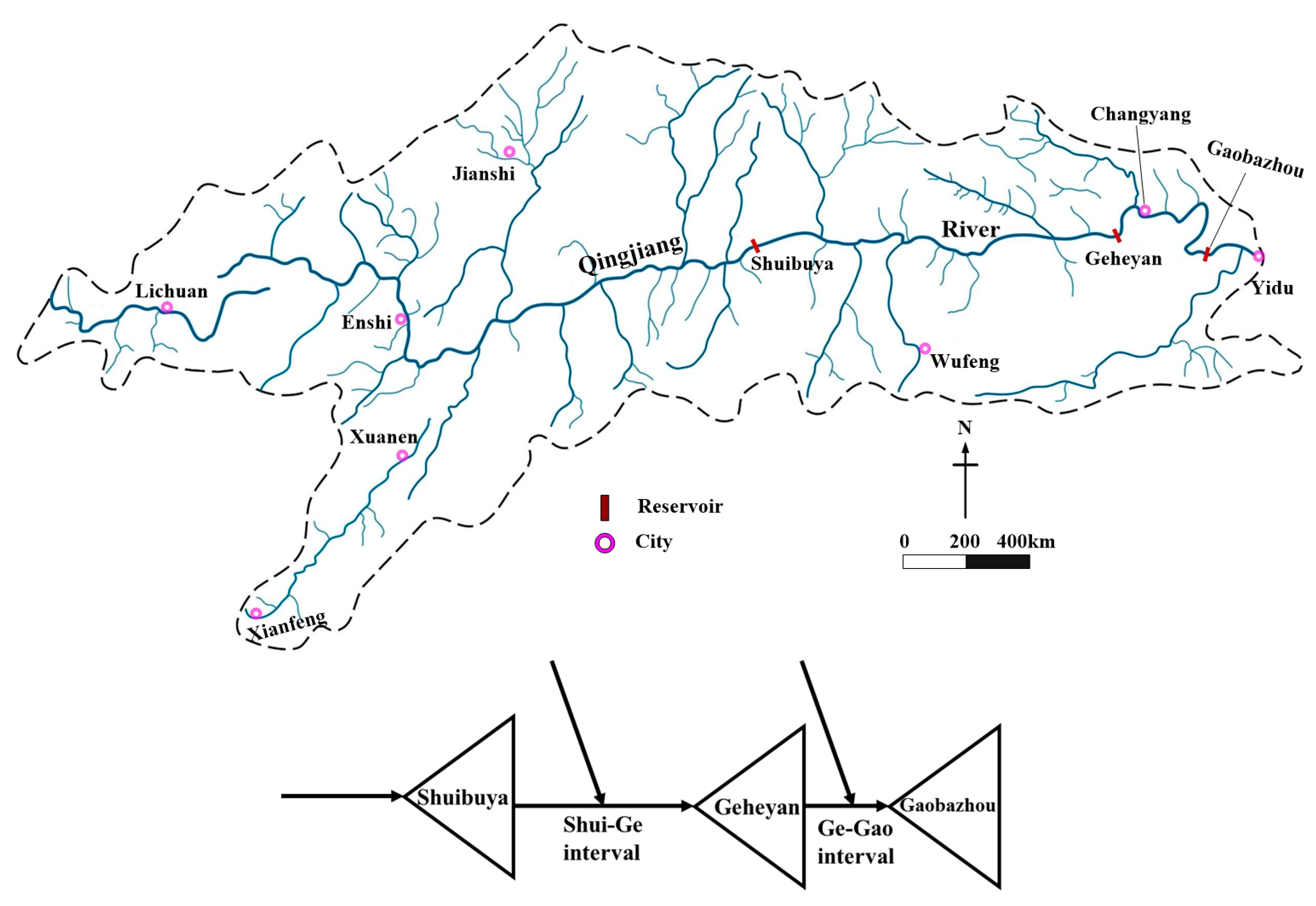
To exemplify the proposed methods, the Qingjiang cascade reservoirs in China are selected. As shown in Figure 2, the Qingjiang River is one of the main tributaries of Yangtze River with a basin area of 17,000 km2. The mean annual rainfall, runoff depth, and annual average discharge are approximately 1460 mm, 876 mm, and 423 m3/s, respectively. The total length of the mainstream is 423 km with a hydraulic drop of 1430 m.
Along the Qingjiang River, a three-step cascade (Shuibuya, Geheyan, and Gaobazhou) reservoir has been constructed from upstream to downstream. The characteristic parameter values of these three reservoirs are given in Table 1. The areas of the two interval basins, one is between Shuibuya and Geheyan reservoirs (Shui-Ge interval basin), and the other is between Geheyan and Gaobazhou reservoirs (Ge-Gao interval basin), are 3570 km2 and 1220 km2, respectively. In this case study, design floods of the Gaobazhou reservoir site are estimated under the impact of Geheyan reservoir and Shuibuya-Geheyan cascade reservoirs operation, respectively; and, the results are compared with those of the natural condition to quantitatively evaluate the impact of upstream reservoirs.
4.1. Natural River Flow Discharge Data Series
A common problem in the statistical analysis of river flow discharges is that watershed changes have occurred during the period of record so that values reflect a nonstationary condition. If the changes are mainly due to the construction of reservoirs, it is possible to adjust flow at a downstream gauge to natural condition by routing reservoir holdouts (increments of stored water) to the hydrologic gauge station adding the routed discharge to the observed discharge. The water balance equation is used to restore natural flow [11], i.e., the stored water flow discharge of the reservoir is
where V(t) and V(t, 1) are reservoir storages at the end of interval t and t − 1, respectively (m3); Δt is the length of time interval (s); and, QS is the stored water flow discharge (m3/s).
The natural river flow discharge at gauge station is
in which
where QN and QO are the natural and observed river flow discharges at gauge station, respectively (m3/s); QR is the reservoir stored water flow routed to the gauge station by the Muskingum method (m3/s); C1, C2,and C3 are routing coefficients that are defined in terms of Δt, K (storage-time constant), and x (weighting factor), and they can be estimated by the Least Square method. In this study, K and x are eaual to 2 h and 0.45, respectively.
The Shuibuya, Geheyan, and Gaobazhou cascade reservoirs have been built in the year of 2008, 1994, and 2001, respectively. There are three hydrologic gauge stations at these dam sites before the construction of reservoir, where the river flow discharge are observed. Therefore, the natural river flow discharge data series (from 1965 to 2010 with 3 h time interval) are restored and obtained by the above method.
There is no flow gauge station in the interval areas and the lateral flow is estimated by water balance equation and the Muskingum routing method. Taking the Shui-Ge inter-basin as an example, the lateral flow Qsg is estimated by
where Qs and Qg are the natural river flows of Shuibuya and Geheyan dam sites, respectively. Qs~g represents the natural river flow discharge at the Shuibuya dam site that was routed to the Geheyan dam site by the Muskingum routing method [44,45].
The procedure introduced above is a standard procedure used in China for restoring river flow discharge data influenced by upstream reservoir. The data used in this study were provided by the Bureau of Hydrology of Yangtze River Water Resources Commission. They are reliable and have been widely used in the planning, design, operation, and management of water resources in the Qingjiang River basin.
4.2. Operation Rules of Shuibuya and Geheyan Reservoirs
As shown in Table 1, the flood limited water level (FLWL) of the Shuibuya and Geheyan reservoirs during flood season are 391.8 m and 192.2 m (a.m.s.l.), respectively. The flood control operation rules of Shuibuya reservoir are described, as follows [46,47]:
- (1)
- If the inflow discharge is less than or equal to the design peak flow with probability 5% (the return period is 20 years), then the reservoir water level is controlled within 397 m (a.m.s.l.);
- (2)
- If the inflow discharge is greater than the design peak discharge with a probability of 5% (the return period is 20 years), but less than the spillway capacity, then the reservoir outflow equals to the inflow; otherwise, the reservoir outflow equals to the spillway capacity.
- (1)
- If the inflow discharge is less than or equal to 11,000 m3/s, then the outflow of reservoir equals to the inflow;
- (2)
- If the inflow discharge is larger than 11,000 m3/s and reservoir water level is less than 200.0 m (a.m.s.l.), then the outflow of reservoir is controlled within 11,000 m3/s;
- (3)
- When the reservoir water level has reached 200.0 m (a.m.s.l.), if the inflow discharge is less than or equal to 13,000 m3/s, then the outflow of reservoir is equal to the inflow; if the inflow discharge is larger than 13,000 m3/s and the reservoir water level is less than 203.0 m (a.m.s.l.), then the outflow of reservoir is controlled within 13,000 m3/s; and,
- (4)
- When the reservoir water level has reached 203.0 m (a.m.s.l.), if the inflow discharge is larger than 13,000 m3/s and less than the spillway capacity, then the outflow of reservoir is equal to the inflow; otherwise, the outflow of the reservoir is equal to the spillway capacity.
4.3. Estimation of Marginal Distributions
According to the regulation characteristics of Shuibuya-Geheyan cascade reservoirs, three-day natural flood volumes (W3) at Shuibuya, Geheyan, and Gaobazhou reservoir sites, Shui-Ge and Ge-Gao inter-basins, and natural peak flow (Qm) at Gaobazhou reservoir site are all i.i.d. random variables and are assumed to follow P3 distributions. The parameters of these six P3 distributions are estimated by the curve-fitting method [3], and the results are listed in Table 2. A Chi-Square Goodness-of-fit test is performed to test the assumption, H0, that the flood magnitudes follow the P3 distribution. Table 2 shows that the assumption could not be rejected at the 5% significance level.
4.4. Determinations of Joint Distributions
To study the impact of the Geheyan reservoir, both the CERC method and MLRC method need the (a) bivariate distribution of W3 at Geheyan reservoir site and Ge-Gao inter-basin. To study the impact of Shuibuya-Geheyan cascade reservoirs, CERC method needs (b) bivariate distributions of W3 at Shuibuya reservoir site and Shui-Ge inter-basin, and (c) bivariate distributions of W3 at the Shuibuya reservoir site and Ge-Gao inter-basin. While MLRC method needs, the (d) trivariate distribution of W3 at the Shuibuya reservoir site, Shui-G and Ge-Gao inter-basins. In this case study, these four (one for single reservoir and three for cascade reservoirs) joint distributions are used and are constructed using the GH copula functions, respectively.
Dependence parameters of the four joint distributions are estimated using Equation (9) or maximum likelihood method that is based on the observed data from 1965 to 2010 and the results are listed in Table 3. The Cramer-von Mises test is used to measure the goodness of fit of the copula distribution. The p-values of the four joint distributions are calculated and also listed in Table 3. It is illustrated from Table 3 that the assumption that variables (a) (b) (c), and (d) follow GH copula function cannot be rejected at 5% significance level with p-values that are all larger than 0.05.
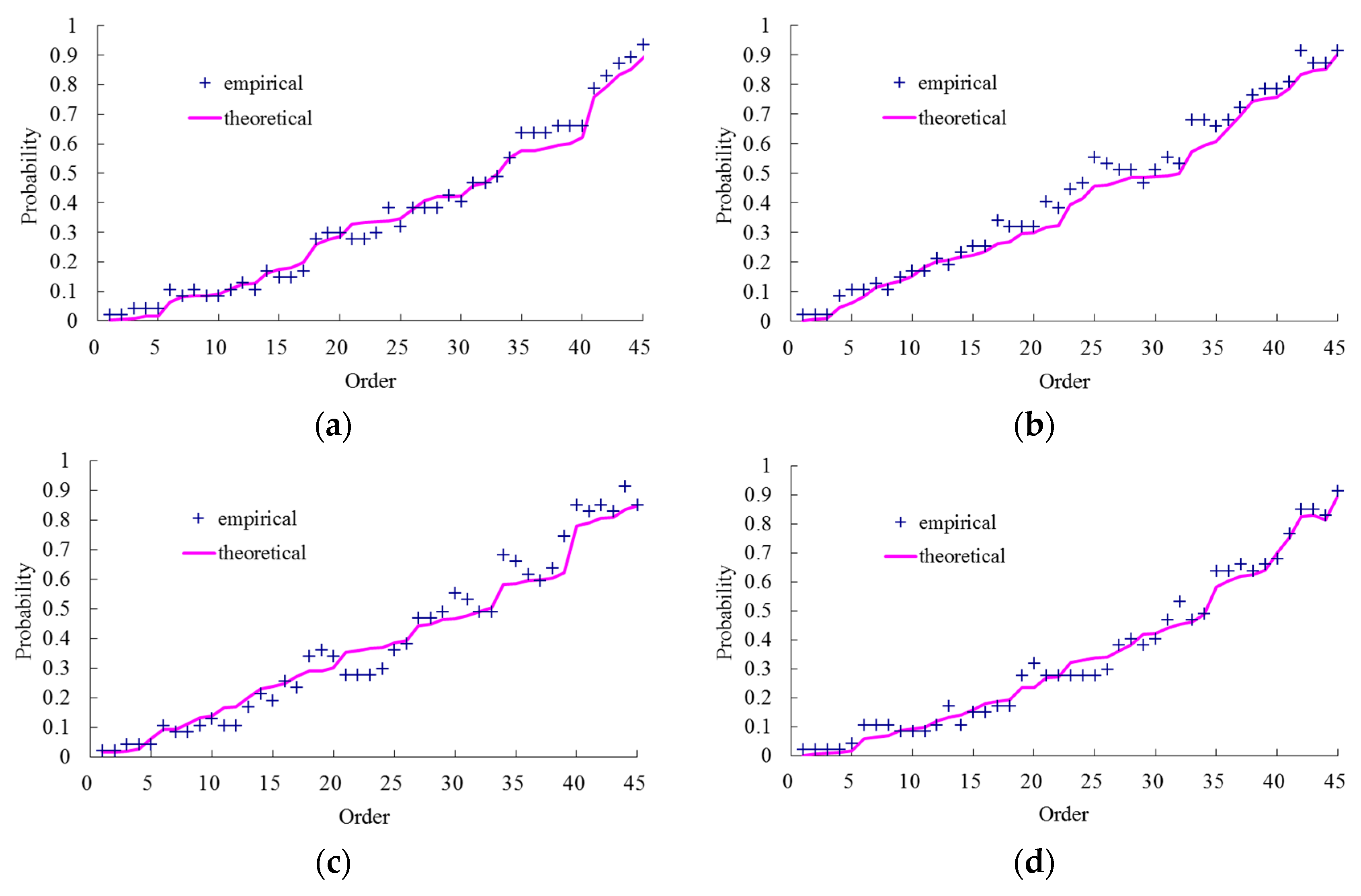
In flood frequency analysis, the Pearson type III distribution and the curve fitting method have been recommended by the Ministry of Water Resources, China [3]. Here, we plot empirical and theoretical joint CDFs to test the fitting ability. A two-dimensional table is constructed in which the variables X and Y are arranged in ascending order. The empirical joint CDF (Pei) can be computed by the Gringorten plotting-position formula [23]:
where Lm,n is the number of occurrences of the combinations of xi and yi.
Likewise, a three-dimensional table also can be constructed in which the variables X, Y and Z are arranged in ascending order. The empirical joint CDF also can be computed by the Gringorten plotting-position formula [25]:
where Tm,n,r is the number of occurrences of the combinations of xi, yj, and zk.
The empirical joint CDFs calculated by Equations (41) and (42) and theoretical values for four joint CDFs that are mentioned above are plotted in Figure 3, which show an overall satisfactory agreement of between the empirical and theoretical joint CDFs.
4.5. The Impact of Geheyan Reservoir Operation
The EFRC, CERC, and MLRC methods for single reservoir were used to analyse flood regional composition of Geheyan reservoir site and Ge-Gao interval basin.
(1) EFRC method
It is assumed that the equivalent frequency floods occur at the Gaobazhou reservoir site and the Geheyan reservoir site, while the corresponding flood occurs at the Ge-Gao interval basin.
(2) CERC method
A given flood occurs at Geheyan reservoir site, while the conditional expected value occurs at Ge-Gao interval basin, and then the conditional expected composition can be determined by the trial and error method.
(3) MLRC method
The maximum value of joint PDF is taken as the objective to determine the most likely composition from the perspective of occurrence probability.
Flood regional compositions of design flood volume at the Gaobazhou reservoir site are calculated based on the three methods mentioned above. Therefore, the three-day flood volume proportions of Geheyan reservoir site and Ge-Gao interval basin are calculated, and the results are listed in Table 4.
It is shown in Table 4 that the proportions of the Ge-Gao interval basin are constant (8.3%) with different design frequencies at the Gaobazhou reservoir site by the EFRC method. The MLRC method exhibits that when flood with return period exceeding 20 years occurs at Gaobazhou reservoir site, the proportions of Geheyan reservoir site range from 89.0% to 89.9%, which is smaller than its proportion of area (92.2%); the proportions of the Ge-Gao inter-basin range from 10.1% to 11.0%, which is larger than its proportion of area (7.8%); it is also shown that the flood volume at the Gaobazhou reservoir site is largely dependent on the flood volume at the Geheyan reservoir site, and the proportion of the Geheyan reservoir site decreases gradually as design flood magnitude at the Gaobazhou reservoir site increases. Generally speaking, the bigger the flood proportion of the Geheyan reservoir site, the larger the impact on design floods at Gaobazhou the reservoir site.
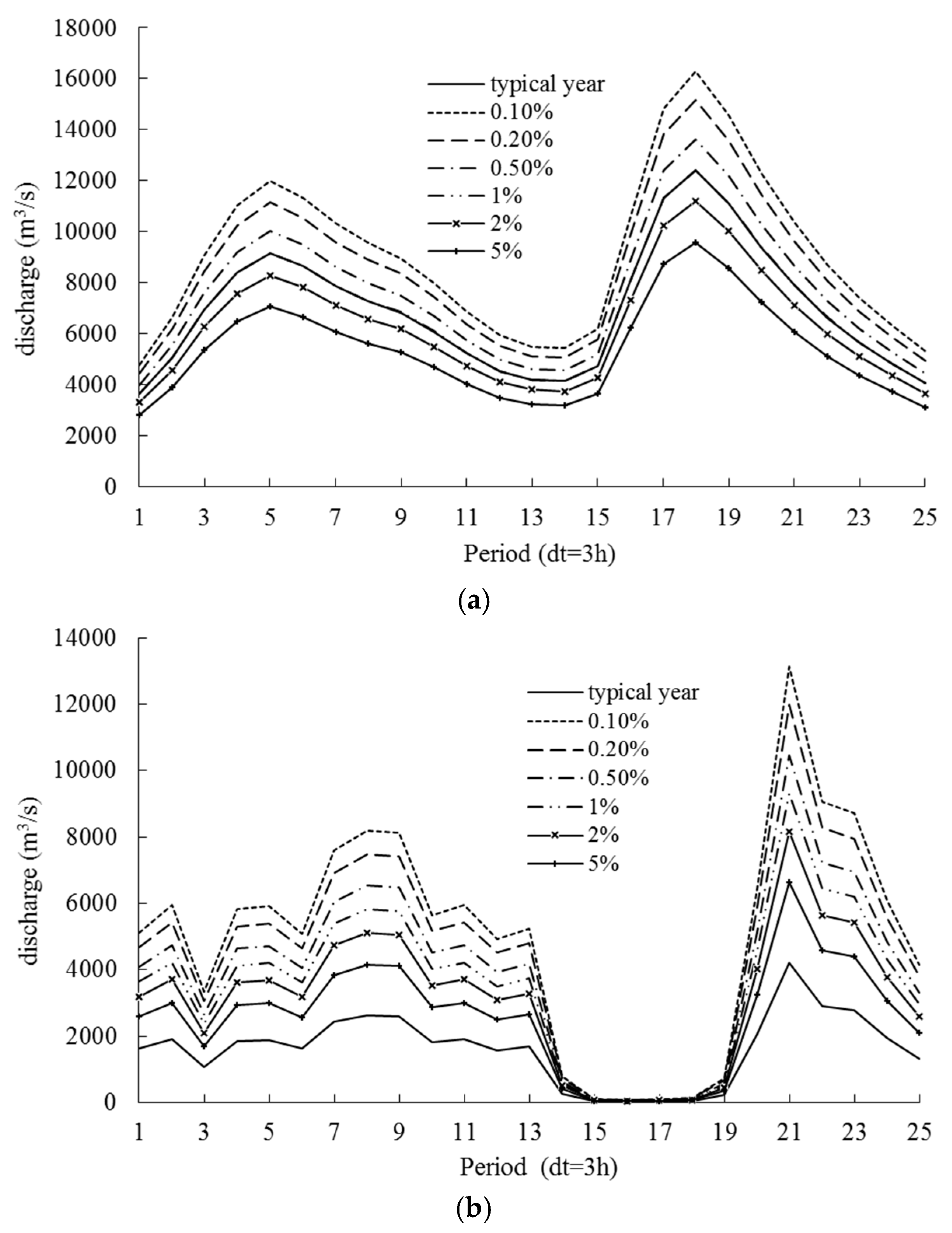
Maximum three-day flood hydrographs in 1997 are selected as the typical floods. The corresponding flood hydrographs with different design frequencies for these three methods at the Geheyan reservoir site and Ge-Gao interval basin are obtained by the same flood amplification ratio [14,15]. Taking the most likely method as an example, the results are plotted in Figure 4.
For each method, the two design flood hydrographs at the Geheyan reservoir site and Ge-Gao inter-basin are routed through the Geheyan reservoir by taking into account of its operation rules (see Figure 4). The peak discharges at the Gaobazhou reservoir site with different return periods by these three methods under the impact of upstream Geheyan reservoir operation are summarized in Table 5, in which the Reduction Rate (RR) calculated by the following equation:
where QN represents the peak discharge under natural condition; QE is the peak discharge estimated by one of these methods (i.e., EFRC, CFRC, and MLRC) under the impact of upstream reservoir operation.
As shown in Table 5, all of the design peak discharges at the Gaobazhou reservoir site have been reduced due to the impact of Geheyan reservoir operation, e.g., for 100-year design values, the reduction ranges from 5360 m3/s to 5900 m3/s. In general, the differences among the methods are not large. For return periods between 20 and 1000 years, the maximum variation of reduction rate among these three methods is about 3.3%. However, the design values of EFRC method are systematically smaller than those of the two methods based on copulas and thus yield an underestimation, which may lead to an increased risk in the hydrological design.
The CFRC and MLRC methods can better capture the spatial correlation of floods that occurred at the Geheyan reservoir site and the Ge-Gao inter-basin. Thus, these two methods with stronger statistical basis are found more reasonable to estimate design floods under the influence of Geheyan reservoir operation.
4.6. Impact of Shuibuya-Geheyan Cascade Reservoirs Operation
Similarly, these three methods were used to analyse flood regional compositions of the Shuibuya reservoir site, Shui-Ge and Ge-Gao inter-basins.
(1) EFRC method
It is assumed that the equivalent frequency floods occur at the Gaobazhou reservoir site and the Geheyan reservoir site, the corresponding flood occurs at Ge-Gao inter-basin; while the equivalent frequency floods also occur at Shuibuya reservoir site and Geheyan reservoir site, and the corresponding flood occurs at Shui-Ge inter-basin.
(2) CERC method
A given flood occurs at Shuibuya reservoir site, while the conditional expected values occur at the Shui-Ge and Ge-Gao inter-basins, respectively. Then, the conditional expected composition can also be determined by the trial and error method.
(3) MLRC method
The maximum value of joint PDF is taken as the objective to determine the most likely composition from the perspective of probability occurrence.
Flood regional compositions of design flood volume at the Gaobazhou reservoir site are calculated based on these three methods mentioned above. Therefore, the three-day flood volume proportions of Shuibuya reservoir site, Shui-Ge and Ge-Gao inter-basins are calculated and the results are listed in Table 6.
It is seen from Table 6 that the proportions of Ge-Gao inter-basin are constant (8.3%) with different design frequencies at the Gaobazhou reservoir site by the EFRC method. This consequence occurs because of the unreasonable assumption in the traditional EFRC method. The control area of Ge-Gao interval basin is 1220 km2, constituting 7.8% of the control area of the Gaobazhou reservoir. In addition, the design floods of the Geheyan and Gaobazhou reservoirs are both based on the Changyang hydrological gauge station. The P3 parameters for annual maximum W3 series for Geheyan and Gaobazhou reservoir are quite similar with scale and shape parameters almost equal to each other (Table 2). Therefore, their design floods almost change by ratio and the proportions of Ge-Gao interval basin are approximately constant (8.3%) and independent of the design frequency under the equivalent frequency assumption. Results of the MLRC method exhibit that when flood with return period exceeding 20 years at Gaobazhou reservoir site occurs, the proportions of Shuibuya reservoir site range from 57.4% to 61.1%, which is smaller than its proportion of area (69.4%); the proportions of Shui-Ge inter-basin range from 29.2% to 31.8%, which is larger than its proportion of area (22.8%); the proportions of Ge-Gao inter-basin range from 9.7% to 10.8%, which is larger than its proportion of area (7.8%). It is also shown that the floods at the Gaobazhou reservoir site are mainly dependent on the floods at Shuibuya reservoir site, and the proportion of the Shuibuya reservoir site decreases gradually with the increase of the design flood magnitude at the Gaobazhou reservoir site.
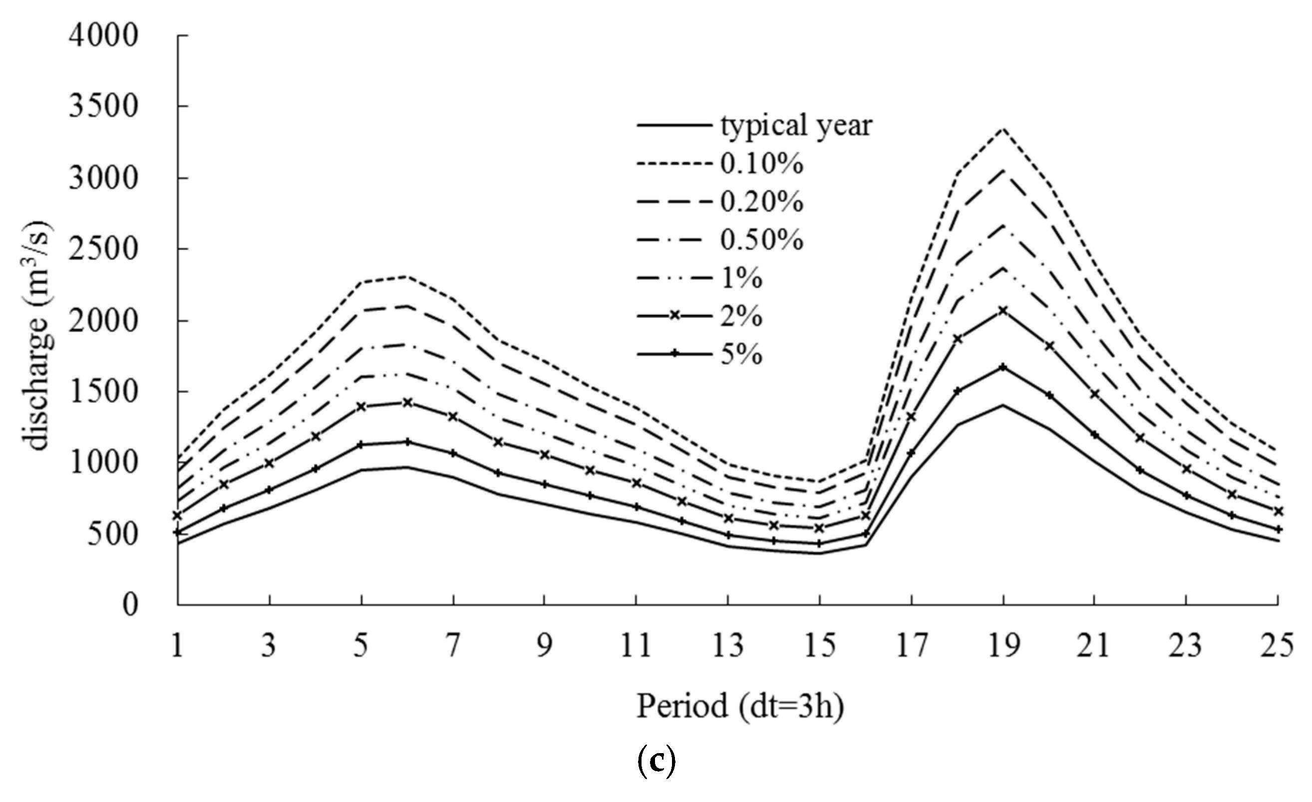
Maximum three-day flood hydrographs in 1997 are selected as the typical floods. The corresponding flood hydrographs with different design frequencies for the three methods at the Shuibuya reservoir site, Shui-Ge and Ge-Gao inter-basins are obtained by the same flood amplification ratio. Taking the MLRC method as an example, the results are plotted in Figure 5.
For each method, the three design flood hydrographs at the Shuibuya reservoir site, Shui-Ge and Ge-Gao inter-basins are routed through the Shuibuya-Geheyan cascade reservoirs by taking into account of their respective operation rules (see Figure 5). The flow hydrographs at Gaobazhou reservoir site are derived and the peak discharges under the influence of Shuibuya-Geheyan cascade reservoirs operation are obtained.
Peak flows at Gaobazhou reservoir site with different return periods in the natural condition and that estimated by three methods under the influence of Shuibuya-Geheyan cascade reservoirs are summarized in Table 7. The reduction rate (RR), defined by Equation (46), and is also shown in Table 7.
The results in the Table 7 also imply that all of the design peak discharges at the Gaobazhou reservoir site have been reduced due to the impact of the upstream Shuibuya-Geheyan cascade reservoirs operation, e.g., for 100-year design peak flow, the reduction ranges from 6710 m3/s to 6920 m3/s. For return periods between 20- and 1000-year, the maximum variation of reduction rate among these three methods is about 3.0%.
It is found that the design values of EFRC method are smaller than those of the two methods that are based on copulas for return periods of 1000-, 500-, 100-, and 50-year, while greater for return periods of 200- and 20-year. It is suggested that the traditional EFRC method which assumes that the floods occurred at Gaobazhou reservoir site, Geheyan reservoir site and Shuibuya reservoir site are perfectly correlated may lead to an under- or overestimation of the risk in hydrological design. The CERC and MLRC methods have considered the actual spatial correlation of floods occurred at the Shuibuya reservoir site, Shui-Ge and Ge-Gao inter-basins. These two methods with a stronger statistical basis are also more reasonable than the EFRC method for estimating design floods under the impact of the Shuibuya-Geheyan cascade reservoirs operation.
5. Discussion
The design flood estimation results at the Gaobazhou reservoir site under the impact of Geheyan reservoir and Shuibuya-Geheyan cascade reservoirs were analyzed using three different methods. The findings and their implications are discussed, as follows.
The currently used EFRC method that assumes the perfect correlation (i.e., correlation coefficient is equal to 1) between peak floods occurred at one sub-basin and downstream site does not always conform to the actual situation. To overcome this drawback of the EFRC method, the CERC and MLRC methods that loose the assumption of perfect correlation are proposed. Compared with the EFRC method, the CERC and MLRC methods only add correlation coefficients (or parameters) of flood volumes between sub-basins. These parameters can be easily estimated by the available methods [23,28,35]. The proposed methods are found to be more flexible in hydrological design compared with EFRC method.
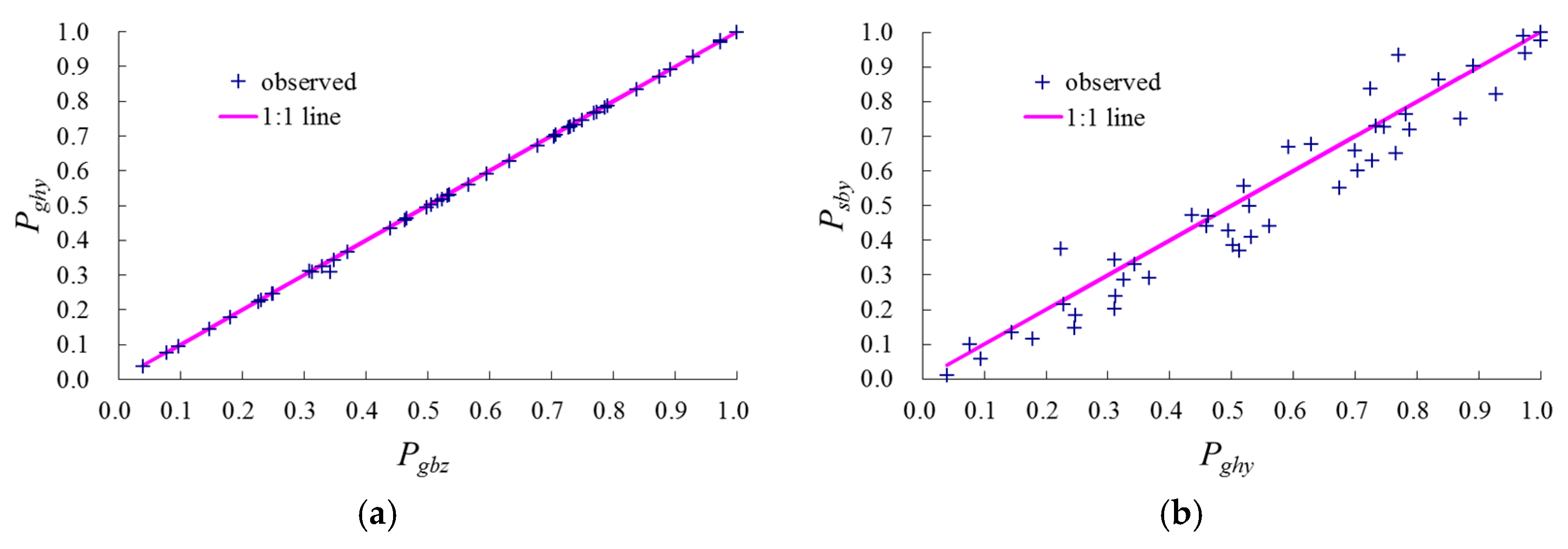
Although no huge differences can be shown from the results estimated by EFRC, CERC, and MLRC methods in this case study, it should be noted that the Qingjiang basin belongs to a middle sized basin that the equivalent frequency flood at each sub-basin is likely to occur with downstream site. Figure 6 shows that differences between Ge-Gao and Shui-Ge inter-basins, on which Psby, Pghy, and Pgbz represent the exceedance probability of 3-day flood volume for Shuibuya, Geheyan and Gaobazhou reservoir sites, respectively. The straight lines show the conditions when exceedance probability of three-day flood volume for Geheyan and Gaobazhou, Shuibuya and Geheyan are identical, respectively. It is seen that the equivalent frequency floods at Geheyan and Gaobazhou reservoir sites are more likely to occur in comparing with the Shuibuya and Geheyan reservoir sites. This difference is due to that the area proportion of Ge-Gao inter-basin (7.8%) is smaller than that of Shui-Ge inter-basin (24.7%). The difference of results for these methods will be increased as the proportion of the inter-basin area increases.
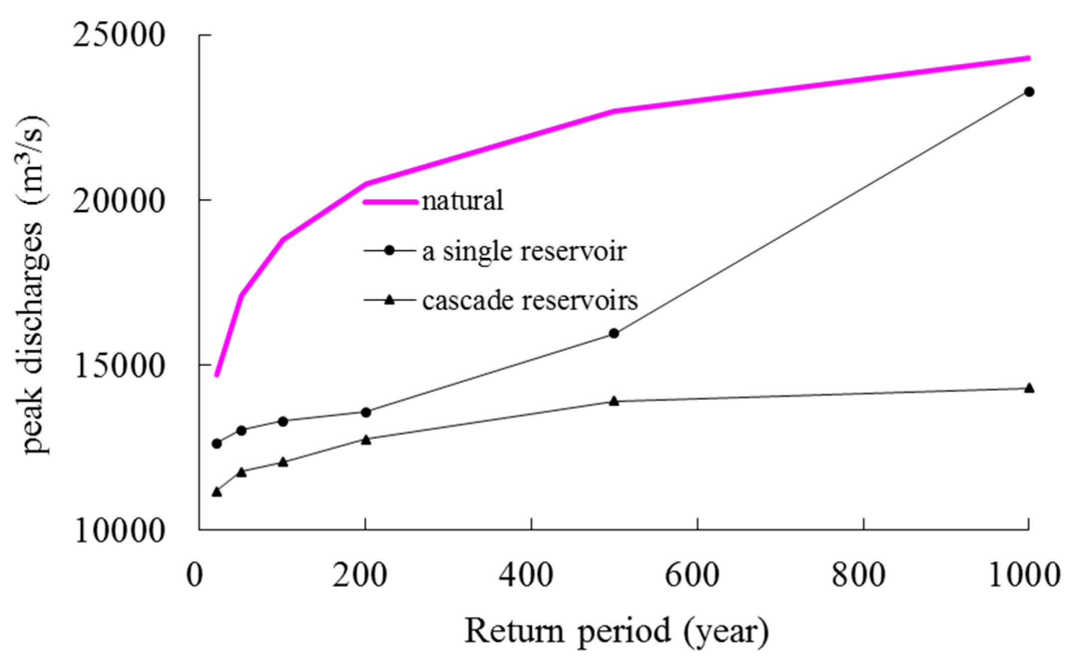
Design floods at the downstream site have been reduced by the regulation of upstream reservoirs as shown in Figure 7. The peak discharges that were estimated at the downstream site involving the joint operation of the cascade reservoirs are reduced much more significantly than those of single reservoir being taken into consideration. For example, 100-year design peak flow (average of three methods) at the Gaobazhou reservoir site is cut by about 35% for cascade reservoirs.
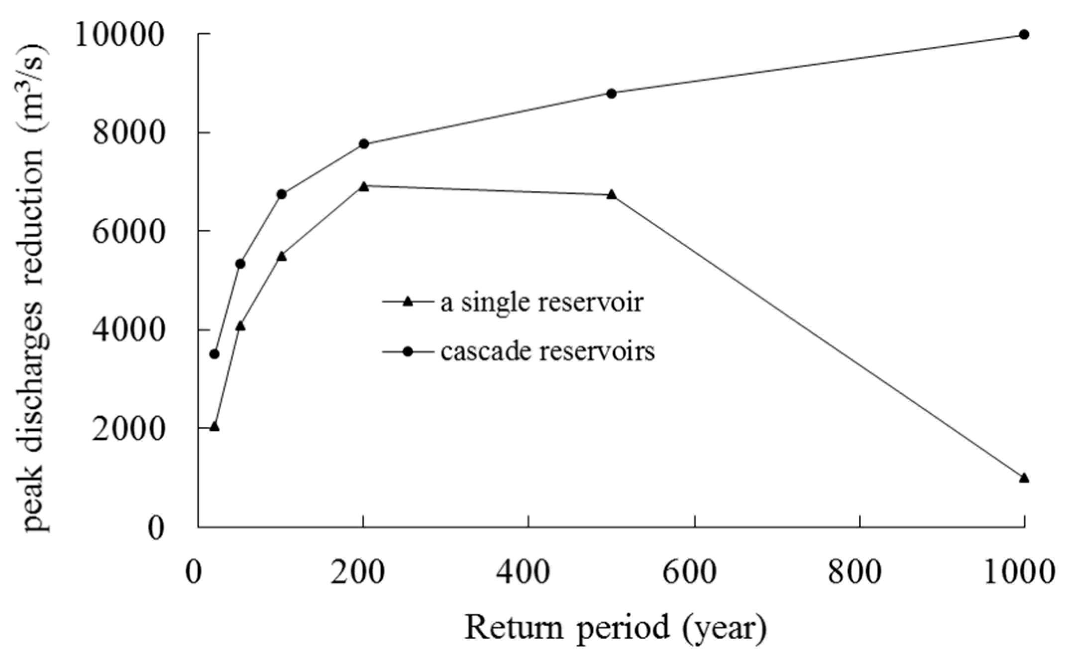
The cutting patterns of estimated peak discharges (average of three methods) at the Gaobazhou reservoir site are different for single and cascade reservoirs. As shown in Figure 8, with the increase of design flood magnitude at the Gaobazhou reservoir site, the reduction curve increases firstly and it then decreases for single reservoir case, and the peak discharge reductions are 2140 m3/s, 7060 m3/s, and 1070 m3/s corresponding with return periods of 20-year, 200-year, and 1000-year, respectively. While the reduction curve increases continuously for the cascade reservoirs and the peak discharge reductions are 3580 m3/s, 7820 m3/s, and 9980 m3/s corresponding with 20-, 200-, and 1000-year return periods, respectively.
6. Conclusions
Reservoirs operation alters the natural flow regime at downstream site and thus has a great impact on the design flood values. The operation rules of the upstream reservoirs should be involved in estimating downstream design floods. In this study, two new flood regional composition methods, i.e., the CERC method and MLRC method both for single reservoir and cascade reservoirs were proposed and developed based on copulas. The Shuibuya-Geheyan- Gaobazhou cascade reservoirs located at the Qingjiang River basin were selected as the case study and the design flood estimation results of the proposed methods were compared with those of the traditional EFRC method. The main conclusions are summarized as follows:
- (1)
- Design peak discharges at the Gaobazhou reservoir site have been reduced significantly due to the impact of upstream reservoirs operation when compared with those in the natural condition. Moreover, the impact of Shuibuya-Geheyan cascade reservoirs is greater than that of only Geheyan reservoir being taken into consideration.
- (2)
- The comparison between the current EFRC method and the proposed CERC and MLRC methods that were based on copulas demonstrates that the EFRC method not taking the actual dependence of floods occurred at various sub-basins into account; as a consequence, it yields an under-or overestimation of the risk that is associated with a given event in hydrological design. Moreover, when the control area of the inter basin is relatively small, the EFRC may lead to unreasonable results due to the perfect correlation assumption between flood events occurred at sub-basin and downstream site. The new methods with stronger statistical basis overcome the main drawback of EFRC method and can better capture the actual spatial correlation of flood events that occurred at various sub-basins, and the estimated design flood values are more reasonable than the currently used EFRC method.
- (3)
- The EFRC method can only be applied step by step to complex cascade reservoirs system, which is not only difficult to implement, but also subjective to some degree. As the number of cascade reservoirs (n) increases, the number of EFRCs (2n) will increase dramatically. Therefore, the MLRC method is recommended for design flood estimation in the complex cascade reservoirs since its composition is unique and easily implementable.
Author Contributions
This research presented here was carried out in collaboration between all authors. Shenglian Guo proposed the methods and wrote the paper. Muhammad Rizwan, Zhangjun Liu, Feng Xiong, Jiabo Yin did computation and analysis work. All authors discussed the results and the manuscript.
Funding
This research was funded by the National Natural Science Foundation of China (NSFC 51539009).
Acknowledgments
The authors would like to thank the editor and anonymous reviewers whose comments and suggestions help to improve the manuscript.
Conflicts of Interest
The authors declare no conflict of interest.
References
- Maidment, D.R. Handbook of Hydrology; McGraw-Hill: New York, NY, USA, 1993. [Google Scholar]
- Guo, S.L.; Zhang, H.G.; Chen, H.; Peng, D.Z.; Liu, P.; Pang, B. A reservoir flood forecasting and control system for China. Hydrol. Sci. J. 2004, 49, 959–972. [Google Scholar] [CrossRef]
- Ministry of Water Resources (MWR). Guidelines for Calculating Design Flood of Water Resources and Hydropower Projects; Chinese Water Resources and Hydropower Press: Beijing, China, 2006. (In Chinese) [Google Scholar]
- Apollonio, C.; Balacco, G.; Gioia, A.; Iacobellis, V.; Piccinni, A.F. Flood hazard assessment of the Fortore river downstream the Occhito Dam in Southern Italy. Comput. Sci. Appl. 2017, 10405, 201–216. [Google Scholar]
- Cunnane, C. Statistical distribution for flood frequency analysis. WMO Oper. Hydrol. Rep. 1989, 33, 73. [Google Scholar]
- US Water Resources Council (USWRC). Guidelines for Determining Flood Flow Frequency; USWRC: Washington, DC, USA, 1981. [Google Scholar]
- Robson, A.; Reed, D. Statistical procedure for flood frequency estimation. In Flood Estimation Handbook (FEH); Institute of Hydrology: Wallingford, UK, 1999; Volume 3. [Google Scholar]
- Yu, Z.; Pollard, D.; Cheng, L. On continental-scale hydrologic simulations with a coupled hydrologic model. J. Hydrol. 2006, 331, 110–124. [Google Scholar] [CrossRef]
- Isik, S.; Dogan, E.; Kalin, L.; Sasal, M.; Agiralioglu, N. Effects of anthropogenic activities on the Lower Sakarya River. Catena 2008, 75, 172–181. [Google Scholar] [CrossRef]
- Duan, W.X.; Guo, S.L.; Wang, J.; Liu, D.D. Impact of Cascaded Reservoirs Group on Flow Regime in the Middle and Lower Reaches of the Yangtze River. Water 2016, 8, 218. [Google Scholar] [CrossRef]
- U.S. Army Corps of Engineers. Flood-Runoff Analysis; EM 1110-2-1417; U.S. Army Corps of Engineers: Washington, DC, USA, 1994. [Google Scholar]
- Favre, A.C.; Adlouni, S.E.; Perreault, L.; Thiémonge, N.; Bobée, B. Multivariate hydrological frequency analysis using copulas. Water Resour. Res. 2004, 40, 290–294. [Google Scholar] [CrossRef]
- Lu, B.; Gu, H.; Xie, Z.; Liu, J.; Ma, L.; Lu, W. Stochastic simulation for determining the design flood of cascade reservoir systems. Hydrol. Res. 2012, 43, 54–63. [Google Scholar] [CrossRef]
- Yue, S.; Ouarda, T.B.; Bobée, B.; Legendre, P.; Bruneau, P. Approach for describing statistical properties of flood hydrograph. J. Hydrol. Eng. 2002, 7, 147–153. [Google Scholar] [CrossRef]
- Xiao, Y.; Guo, S.L.; Chen, L. Design flood hydrograph based on multi-characteristic synthesis index method. J. Hydrol. Eng. 2009, 14, 1359–1364. [Google Scholar] [CrossRef]
- Boughton, W.; Droop, O. Continuous simulation for design flood estimation—A review. Environ. Model. Softw. 2003, 18, 309–318. [Google Scholar] [CrossRef]
- Nijssen, D.; Schumann, A.; Pahlow, M.; Klein, B. Planning of technical flood retention measures in large river basins under consideration of imprecise probabilities of multivariate hydrological loads. Nat. Hazards Earth Syst. Sci. 2009, 9, 1349–1363. [Google Scholar] [CrossRef]
- De Michele, C.; Salvadori, G. A Generalized Pareto intensity-duration model of storm rainfall exploiting 2-Copulas. J. Geophys. Res. 2003, 108. [Google Scholar] [CrossRef]
- Salvadori, G.; De Michele, C. Frequency analysis via copulas: Theoretical aspects and applications to hydrological events. Water Resour. Res. 2004, 40, 229–244. [Google Scholar] [CrossRef]
- Salvadori, G.; De Michele, C.; Durante, F. On the return period and design in a multivariate framework. Hydrol. Earth Syst. Sci. 2011, 15, 3293–3305. [Google Scholar] [CrossRef] [Green Version]
- Salvadori, G.; Durante, F.; De Michele, C.; Bernardi, M.; Petrella, L. A multivariate Copula-based framework for dealing with Hazard Scenarios and Failure Probabilities. Water Resour. Res. 2016, 52, 3701–3721. [Google Scholar] [CrossRef]
- Grimaldi, S.; Serinaldi, F. Asymmetric copula in multivariate flood frequency analysis. Adv. Water. Resour. 2006, 29, 1155–1167. [Google Scholar] [CrossRef]
- Zhang, L.; Singh, V.P. Bivariate flood frequency analysis using the copula method. J. Hydrol. Eng. 2006, 11, 150–164. [Google Scholar] [CrossRef]
- Zhang, L.; Singh, V.P. Bivariate rainfall frequency distributions using Archimedean copulas. J. Hydrol. 2007, 332, 93–109. [Google Scholar] [CrossRef]
- Zhang, L.; Singh, V.P. Gumbel-Hougaard copula for trivariate rainfall frequency analysis. J. Hydrol. Eng. 2007, 12, 409–419. [Google Scholar] [CrossRef]
- Zhang, L.; Singh, V.P. Trivariate flood frequency analysis using the Gumbel-Hougaard copula. J. Hydrol. Eng. 2007, 12, 431–439. [Google Scholar] [CrossRef]
- Bárdossy, A.; Li, J. Geostatistical interpolation using copulas. Water Resour. Res. 2008, 44, W07412. [Google Scholar] [CrossRef]
- Genest, C.; Favre, A.C. Everything you always wanted to know about copula modeling but were afraid to ask. J. Hydrol. Eng. 2007, 12, 347–368. [Google Scholar] [CrossRef]
- Serinaldi, F.; Bonaccorso, B.; Cancelliere, A.; Grimaldi, S. Probabilistic characterization of drought properties through copulas. Phys. Chem. Earth 2009, 34, 596–605. [Google Scholar] [CrossRef]
- De Michele, C.; Salvadori, G.; Canossi, M.; Petaccia, A.; Rosso, R. Bivariate statistical approach to check adequacy of dam spillway. J. Hydrol. Eng. 2005, 10, 50–57. [Google Scholar] [CrossRef]
- Chen, L.; Singh, V.P.; Guo, S.L.; Hao, Z.C.; Li, T.Y. Flood coincidence risk analysis using multivariate copula functions. J. Hydrol. Eng. 2012, 17, 742–755. [Google Scholar] [CrossRef]
- Li, T.Y.; Guo, S.L.; Liu, Z.J.; Xiong, L.H.; Yin, J.B. Bivariate design flood quantile selection using copulas. Hydrol. Res. 2017, 48, 997–1013. [Google Scholar] [CrossRef]
- Yin, J.B.; Guo, S.L.; Liu, Z.J.; Yang, G.; Zhong, Y.X.; Liu, D.D. Uncertainty analysis of bivariate design flood estimation and its impacts on reservoir routing. Water Resour. Manag. 2018, 32, 1795–1809. [Google Scholar] [CrossRef]
- Sklar, A. Fonctions de repartition an dimensions et leurs marges. Publ. Inst. Stat. Univ. Paris 1959, 8, 229–231. [Google Scholar]
- Nelsen, R.B. An Introduction to Copulas, 2nd ed.; Springer: New York, NY, USA, 2006. [Google Scholar]
- Strupczewski, W.G.; Singh, V.P.; Feluch, W. Non-stationary approach to at-site flood frequency modelling I. Maximum likelihood estimation. J. Hydrol. 2001, 248, 123–142. [Google Scholar] [CrossRef]
- Genest, C.; Huang, W.; Dufour, J.-M. A regularized goodness-of-fit test for copulas. J. Soc. Franc. Stat. 2013, 154, 64–77. [Google Scholar]
- Genest, C.; Rémillard, B.; Beaudoin, D. Goodness-of-fit tests for copulas: A review and a power study. Insur. Math. Econ. 2009, 44, 199–214. [Google Scholar] [CrossRef]
- Pesarin, F. Multivariate Permutation Tests: With Applications in Biostatistics; Wiley: Hoboken, NJ, USA, 2001. [Google Scholar]
- Chebana, F.; Quarda, T.B.M.J. Multivariate quantiles in hydrological frequency analysis. Environmetrics 2011, 22, 63–78. [Google Scholar] [CrossRef]
- Salvadori, G.; De Michele, C. On the use of copulas in hydrology: Theory and practice. J. Hydrol. Eng. 2007, 12, 369–380. [Google Scholar] [CrossRef]
- Gräler, B.; van den Berg, M.J.; Vandenberghe, S.; Petroselli, A.; Grimaldi, S.; Baets, B.D.; Verhoest, N.E.C. Multivariate return periods in hydrology: A critical and practical review focusing on synthetic design hydrograph estimation. Hydrol. Earth Syst. Sci. 2013, 17, 1281–1296. [Google Scholar] [CrossRef] [Green Version]
- Li, T.Y.; Guo, S.L.; Chen, L.; Guo, J.L. Bivariate flood frequency analysis with historical information based on Copula. J. Hydrol. Eng. 2013, 18, 1018–1030. [Google Scholar] [CrossRef]
- Das, A. Parameter estimation for Muskingum models. J. Irrig. Drain. Eng. 2004, 130, 140–147. [Google Scholar] [CrossRef]
- Birkhead, A.L.; James, C.S. Muskingum River routing with dynamic bank storage. J. Hydrol. 2002, 264, 113–132. [Google Scholar] [CrossRef]
- Guo, S.L.; Chen, J.H.; Li, Y.; Liu, P.; Li, T.Y. Joint operation of the multi-reservoir system of the Three Gorges and the Qingjiang cascade reservoirs. Energies 2011, 4, 1036–1050. [Google Scholar] [CrossRef]
- Chen, J.H.; Guo, S.L.; Li, Y.; Liu, P.; Zhou, Y.L. Joint operation and dynamic control of flood limiting water levels for cascade reservoirs. Water Resour. Manag. 2013, 27, 749–763. [Google Scholar] [CrossRef]
Figure 1.
Sketch diagrams of natural condition and flood control system. (a) Natural condition; (b) Single reservoir; and, (c) Cascade reservoirs.
Figure 1.
Sketch diagrams of natural condition and flood control system. (a) Natural condition; (b) Single reservoir; and, (c) Cascade reservoirs.

Figure 2.
Sketch maps of the Qingjiang cascade reservoirs.

Figure 3.
Plots of empirical and theoretical values for four joint cumulative distribution functions (CDFs). Note: Order represents number of ordered pair, ranked in the ascending order in terms of theoretical joint CDF, respectively. (a) Geheyan and Ge-Gao inter-basin; (b) Shuibuya and Shui-Ge inter-basin; (c) Shuibuya and Ge-Gao inter-basin; and, (d) Shuibuya, Shui-Ge, and Ge-Gao inter-basins.

Figure 4.
Design inflow hydrographs at two sub-basins for single reservoir. (a) Geheyan basin; and, (b) Ge-Gao inter-basin.
Figure 4.
Design inflow hydrographs at two sub-basins for single reservoir. (a) Geheyan basin; and, (b) Ge-Gao inter-basin.

Figure 5.
Design inflow hydrographs at three sub-basins for cascade reservoirs. (a) Shuibuya basin; (b) Shui-Ge inter-basin; and, (c) Ge-Gao inter-basin.
Figure 5.
Design inflow hydrographs at three sub-basins for cascade reservoirs. (a) Shuibuya basin; (b) Shui-Ge inter-basin; and, (c) Ge-Gao inter-basin.


Figure 6.
Occurrence probability of equivalent frequency floods for sub-basin and downstream site. Note: Psby, Pghy, and Pgbz represent the exceedance probability of three-day flood volume for Shuibuya, Geheyan and Gaobazhou reservoir site, respectively. The straight lines show the conditions when exceedance probability of three-day flood volume for Geheyan and Gaobazhou, Shuibuya and Geheyan are identical, respectively. (a) Geheyan and Gaobazhou reservoir sites; and (b) Shuibuya and Geheyan reservoir sites.

Figure 7.
Comparison of design peak discharges at Gaobazhou reservoir site in the natural condition and those of under the influence of upstream reservoirs operation.
Figure 7.
Comparison of design peak discharges at Gaobazhou reservoir site in the natural condition and those of under the influence of upstream reservoirs operation.

Figure 8.
Design peak discharges reduction at the Gaobazhou reservoir site under the influence of upstream reservoirs operation.
Figure 8.
Design peak discharges reduction at the Gaobazhou reservoir site under the influence of upstream reservoirs operation.


Table 1.
List of characteristic parameter values of the Qinjiang cascade reservoirs.
| Reservoir | Shuibuya | Geheyan | Gaobazhou |
|---|---|---|---|
| Type of dam | Face rock fill dam | Gravity arch dam | Gravity dam |
| Discharging capacity (m3/s) | 18,320 | 23,900 | 22,650 |
| Control area (km2) | 10,860 | 14,430 | 15,650 |
| Total storage (108 m3) | 45.8 | 37.7 | 4.85 |
| Flood control storage (108 m3) | 5.0 | 5.0 | — |
| Flood limited water level (a.m.s.l.) | 391.8 | 192.2 | — |
| Normal water level (a.m.s.l.) | 400.0 | 200.0 | 80.0 |
| Design flood water level (a.m.s.l.) | 402.25 | 203.14 | 80.0 |
| Regulation ability | multi-year | annual | Daily |
Table 2.
Estimated parameters of the P3 marginal distribution for each region.
| Variable | Parameter | Chi-Square Statistics, χ2 | χ0.05 | ||
|---|---|---|---|---|---|
| W3 at Shuibuya reservoir site | 2.30 | 0.43 | 2.65 | 0.738 | 3.841 |
| W3 at Shui-Ge inter-basin | 1.16 | 0.56 | 1.03 | 1.256 | 3.841 |
| W3 at Geheyan reservoir site | 1.85 | 0.25 | 3.70 | 1.646 | 3.841 |
| W3 at Ge-Gao inter-basin | 1.16 | 2.64 | 0.35 | 3.305 | 3.841 |
| W3 at Gaobazhou reservoir site | 1.85 | 0.23 | 4.03 | 2.033 | 3.841 |
| Qm at Gaobazhou reservoir site | 2.78 | 0.0005 | 2773 | 1.341 | 3.841 |
Table 3.
Estimated parameters of the G-H copula function and Cramer-von Mises test.
| Variables | τ | θ/[θ1, θ2] | p-Value |
|---|---|---|---|
| (a) W3 at Geheyan reservoir site and Ge-Gao inter-basin | 0.583 | 2.40 | 0.825 |
| (b) W3 at Shuibuya reservoir site and Shui-Ge inter-basin | 0.468 | 1.88 | 0.507 |
| (c) W3 at Shuibuya reservoir site and Ge-Gao inter-basin | 0.766 | 4.28 | 0.324 |
| (d) W3 at Shuibuya reservoir site, Shui-Ge and Ge-Gao inter-basins | — | [2.11, 4.28] | 0.623 |
Table 4.
Regional three-day flood volume proportions at Gaobazhou reservoir site (%).
| Method | Return Period | 1000 | 500 | 200 | 100 | 50 | 20 |
|---|---|---|---|---|---|---|---|
| Gaobazhou (108 m3) | 42.89 | 39.57 | 35.14 | 31.74 | 28.30 | 23.65 | |
| EFRC | Geheyan reservoir site | 91.7 | 91.7 | 91.7 | 91.7 | 91.7 | 91.7 |
| Ge-Gao inter-basin | 8.3 | 8.3 | 8.3 | 8.3 | 8.3 | 8.3 | |
| CERC | Geheyan reservoir site | 89.8 | 90.0 | 90.2 | 90.5 | 90.7 | 91.1 |
| Ge-Gao inter-basin | 10.2 | 10.0 | 9.8 | 9.5 | 9.3 | 8.9 | |
| MLRC | Geheyan reservoir site | 89.0 | 89.1 | 89.3 | 89.4 | 89.6 | 89.9 |
| Ge-Gao inter-basin | 11.0 | 10.9 | 10.7 | 10.6 | 10.4 | 10.1 |
Table 5.
Peak discharges at Gaobazhou reservoir site with different return periods under the impact of Geheyan reservoir operation (m3/s).
Table 5.
Peak discharges at Gaobazhou reservoir site with different return periods under the impact of Geheyan reservoir operation (m3/s).
| Return Period | QN under Natural Condition | QE under the Impact of Geheyan Reservoir | |||||
|---|---|---|---|---|---|---|---|
| EFRC | RR (%) | CFRC | RR (%) | MLRC | RR (%) | ||
| 1000 | 24,300 | 23,020 | 5.3 | 23,280 | 4.2 | 23,380 | 3.8 |
| 500 | 22,700 | 15,380 | 32.2 | 15,890 | 30.0 | 16,130 | 28.9 |
| 200 | 20,500 | 13,110 | 36.0 | 13,490 | 34.2 | 13,730 | 33.0 |
| 100 | 18,800 | 12,900 | 31.4 | 13,200 | 29.8 | 13,440 | 28.5 |
| 50 | 17,100 | 12,700 | 25.7 | 12,900 | 24.6 | 13,140 | 23.2 |
| 20 | 14,700 | 12,420 | 15.5 | 12,530 | 14.8 | 12,740 | 13.3 |
Table 6.
Proportion of 3-day flood volume in each region at Gaobazhou reservoir site (%).
| Method | Return Period | 1000 | 500 | 200 | 100 | 50 | 20 |
|---|---|---|---|---|---|---|---|
| Gaobazhou (108 m3) | 42.89 | 39.57 | 35.14 | 31.74 | 28.30 | 23.65 | |
| EFRC | Shuibuya reservoir site | 59.1 | 59.4 | 60.0 | 60.4 | 61.0 | 62.0 |
| Shui-Ge inter-basin | 32.6 | 32.3 | 31.7 | 31.3 | 30.7 | 29.7 | |
| Ge-Gao inter-basin | 8.3 | 8.3 | 8.3 | 8.3 | 8.3 | 8.3 | |
| CERC | Shuibuya reservoir site | 59.8 | 60.3 | 61.0 | 61.8 | 62.8 | 64.2 |
| Shui-Ge inter-basin | 29.6 | 29.2 | 28.2 | 27.5 | 26.8 | 25.8 | |
| Ge-Gao inter-basin | 10.6 | 10.5 | 10.8 | 10.7 | 10.4 | 10.0 | |
| MLRC | Shuibuya reservoir site | 57.4 | 57.9 | 58.6 | 59.2 | 59.9 | 61.1 |
| Shui-Ge inter-basin | 31.8 | 31.5 | 31.0 | 30.6 | 30.0 | 29.2 | |
| Ge-Gao inter-basin | 10.8 | 10.6 | 10.4 | 10.2 | 10.1 | 9.7 |
Table 7.
Design peak discharges at Gaobazhou site with different return periods under the impact of Shuibuya-Geheyan cascade reservoirs operation (m3/s).
Table 7.
Design peak discharges at Gaobazhou site with different return periods under the impact of Shuibuya-Geheyan cascade reservoirs operation (m3/s).
| Return Period | QN under Natural Condition | QE under the Impact of Shuibuya-Geheyan Cascade Reservoirs | |||||
|---|---|---|---|---|---|---|---|
| EFRC | RR (%) | CFRC | RR (%) | MLRC | RR (%) | ||
| 1000 | 24,300 | 13,980 | 42.5 | 14,320 | 41.1 | 14,350 | 40.9 |
| 500 | 22,700 | 13,370 | 41.1 | 14,010 | 38.3 | 14,060 | 38.1 |
| 200 | 20,500 | 12,750 | 37.8 | 12,660 | 38.2 | 12,710 | 38.0 |
| 100 | 18,800 | 11,880 | 36.8 | 12,120 | 35.5 | 12,090 | 35.7 |
| 50 | 17,100 | 11,640 | 31.9 | 11,810 | 30.9 | 11,780 | 31.1 |
| 20 | 14,700 | 11,160 | 24.1 | 11,120 | 24.4 | 11,200 | 23.8 |
© 2018 by the authors. Licensee MDPI, Basel, Switzerland. This article is an open access article distributed under the terms and conditions of the Creative Commons Attribution (CC BY) license (http://creativecommons.org/licenses/by/4.0/).
Share and Cite
MDPI and ACS Style
Guo, S.; Muhammad, R.; Liu, Z.; Xiong, F.; Yin, J. Design Flood Estimation Methods for Cascade Reservoirs Based on Copulas. Water 2018, 10, 560. https://doi.org/10.3390/w10050560
AMA Style
Guo S, Muhammad R, Liu Z, Xiong F, Yin J. Design Flood Estimation Methods for Cascade Reservoirs Based on Copulas. Water. 2018; 10(5):560. https://doi.org/10.3390/w10050560
Chicago/Turabian StyleGuo, Shenglian, Rizwan Muhammad, Zhangjun Liu, Feng Xiong, and Jiabo Yin. 2018. "Design Flood Estimation Methods for Cascade Reservoirs Based on Copulas" Water 10, no. 5: 560. https://doi.org/10.3390/w10050560
Note that from the first issue of 2016, this journal uses article numbers instead of page numbers. See further details here.