Numerical Modeling of Long-Term Biogeochemical Processes and Its Application to Sedimentary Bed Formation in Tokyo Bay

Abstract

Even though models of water quality have become increasingly detailed over time, their applicability to analyze long-term effect on sedimentary bed formation is yet to be clarified. Hence, an integrated, layer-resolved, process-based, sediment–water coupled, long-term robust, three-dimensional (3D) ecosystem model, including realistic sedimentary and pelagic processes, was developed. The constituents of the integrated model included a multi layered ecosystem model, a quasi-three dimensional hydrodynamic model, a wave hindcasting model, and a sediment deposition and erosion model. Because numerical modeling difficulties arise in setting the initial conditions, especially for a sedimentary bed, this novel modeling approach suggests to initiate the model with the simplest initial conditions of no particulate organic carbon content (POCC) and uniform inorganic sediment distribution. The model was applied to Tokyo Bay and quasi-steady state POCC in the sediment was obtained through long-term computation with realistic sedimentary and pelagic processes. Wave induced bed shear stress (WBSS) is critical for sediment erosion and spatial movement of sediment pollution, while a stable morphology is determined by the balance between the current induced bed shear stress (CBSS) and WBSS in Tokyo Bay. This novel modeling approach, with the simplest sedimentary initial conditions and realistic sedimentary and pelagic processes, provides a great tool for long-term ecosystem modeling in future studies.

1. Introduction

The occurrence of seasonal hypoxic and anoxic environments in shallow coastal and estuarine waters in the world has increased in the recent past, with the ensuing adverse effects to biodiversity, fisheries, and food webs. Even though observations provide information on coastal and estuarine dynamics to some extent, they are sometimes insufficient for a detailed understanding of water and sediment processes [1], analysis of restoration scenarios, and especially for future predictions on, for instance, the effect of coastal water pollution on climate change [2,3]. In order to fill this gap, with the advancement in computer technology, numerical water quality models have emerged and have been extensively developed over time to understand, analyze, and forecast estuarine and coastal environments and thereby support managerial decision making [4,5,6,7].

Although these models can be used to support water quality management and decision making, they increasingly depend on accurate modeling; hence, models should be more realistic [8,9]. In recent decades, complex descriptions of pelagic biogeochemical effects have been coupled to 3D hydrodynamic models [10,11,12,13]. At the same time, sophisticated, stand-alone, one-dimensional benthic biogeochemical models have been developed [14,15,16], together with some benthic–pelagic coupled models limited to depth integrated [17], two-layer [18,19,20], or layer-resolved models excluding the sedimentary bed formation [19]. However, benthic–pelagic coupled water quality modeling in 3D, with resolved layers and detailed sedimentary and pelagic processes including realistic initial conditions, is still challenging.

It is well-known that water quality depends not only on hydrodynamic forces but also on biogeochemical processes of the ecosystem [21]. Moreover, in shallow estuarine and coastal areas, sediment biogeochemical processes have a strong impact on the overall dynamics of the estuaries and coastal systems, especially on bottom water [17,22,23,24]. Hence, a critical aspect of water quality modeling, particularly for long-term predictions and for considering measures against hypoxia and anoxia, is the accurate estimation of sediment quality. Thus, water quality modeling, especially for long-term predictive models, should include a 3D, layer-resolved, and detailed sediment processes, including sediment bed formation and benthic–pelagic coupling [18,24,25,26].

Tokyo Bay surrounded by the metropolis of Japan with the largest population density and economic accumulation, represents one of the most polluted shallow coastal waters in the world. Red tides [27] occur in the bay and have increased in frequency from spring to autumn with different composition of species, resulting in large quantity of organic material to sediment and severe oxygen depletion in the bottom water [6,28,29,30,31,32]. Moreover, water stratification occurs owing to the warm temperature and fresh water discharge from spring to autumn, thus forming oxygen-depleted bottom water. Wind-induced current causes upwelling of the bottom anoxic water in the bay. Consequently, nutrient rich water moves to the euphotic zone for abnormal phytoplankton production in the surface water [27]. With the inflow of fresh water to the bay, the low-salinity water flows out from the upper layer of the bay, and in compensation, high salinity oceanic water flows into the lower layer forcing the bottom hypoxic water mass towards the head of the bay [33] (estuarine circulation). In addition, Tokyo Bay shows active benthic–pelagic coupling in the inner part of the bay, confirming that benthic–pelagic coupling is tight and active in shallow coastal and shelf areas [23,34].

During the past decades, water quality models of Tokyo Bay have been developed to reproduce its different aspects, which have emerged by data analysis. These aspects include, for instance, some of the physical and ecosystemic characteristics of water and sediment such as upwelling and blue tide [35], the effects of waves and currents on the sediment [36], mud accumulation and bed characteristics [5,37], and seasonal/daily dynamics of water and sediment [6]. However, attempts to reproduce the spatial distributions of water and sediment quality through modeling approaches, which would support the management of water quality in the bay, are scarce or neglected. Meanwhile, the data show higher sediment water content (WC) at the inner part of the bay with a correlation to the sediment POCC [38,39], which in turn affects water quality deterioration.

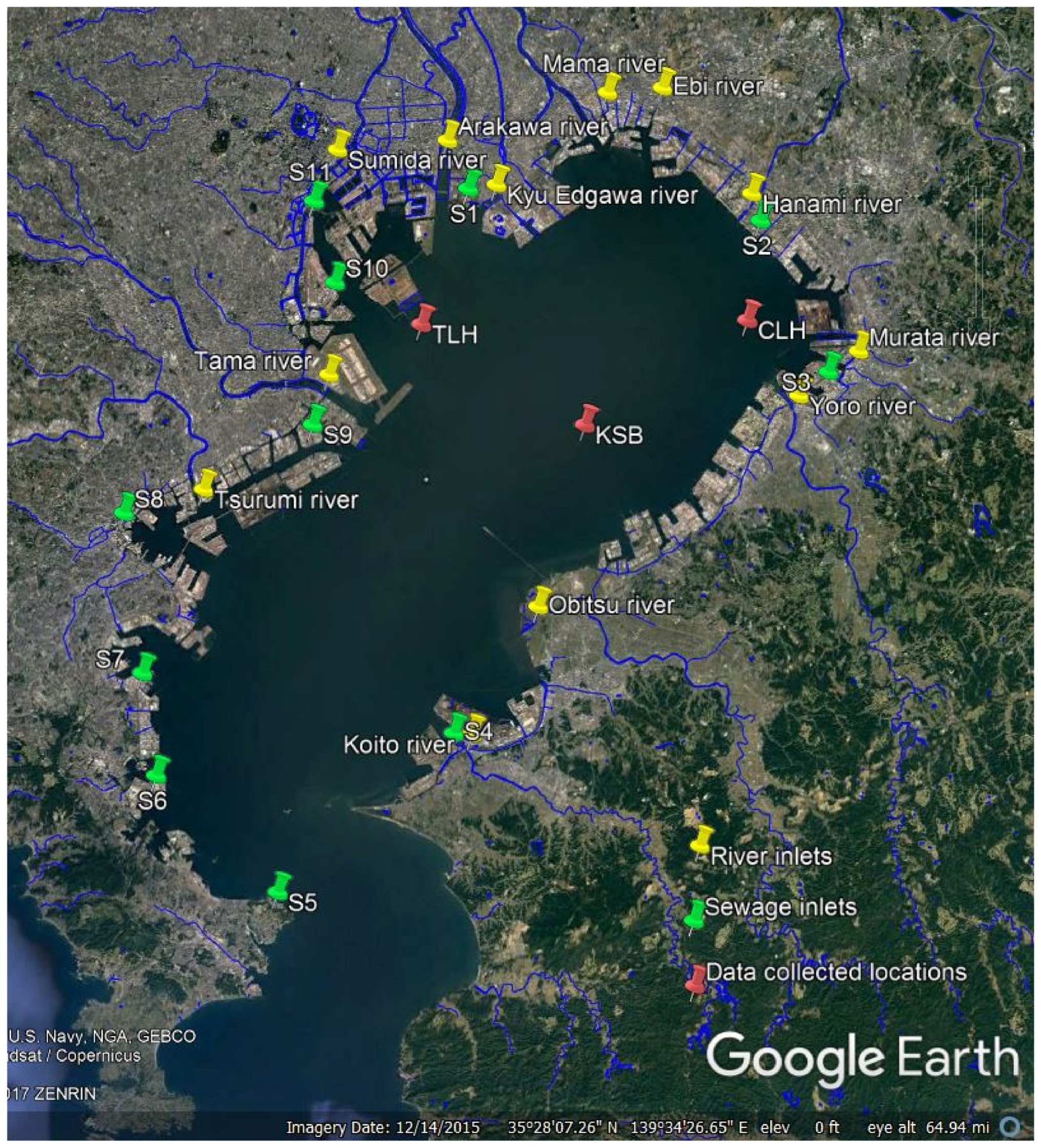
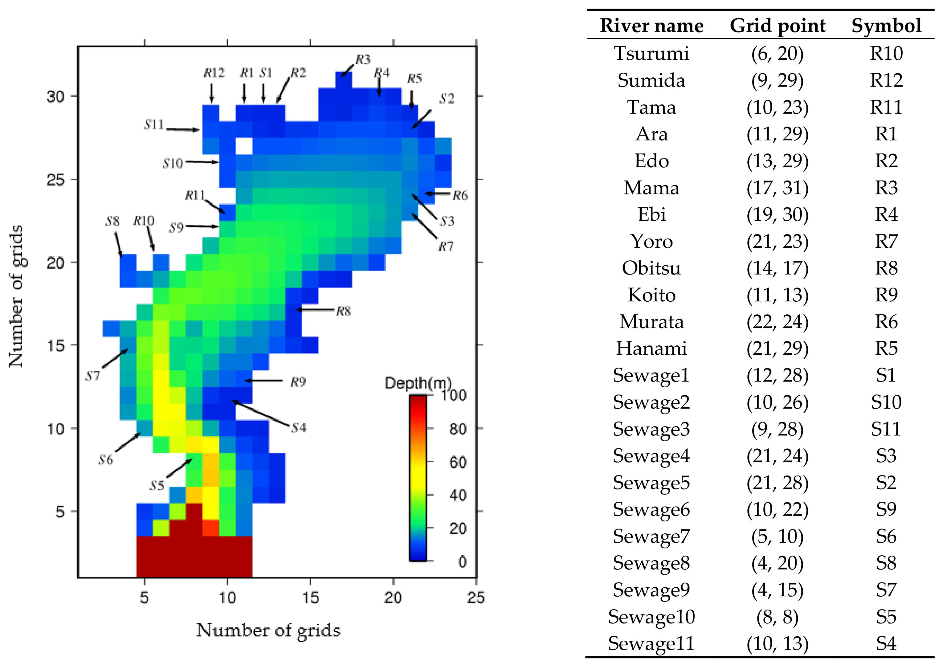
We have been developing a benthic–pelagic coupled 3D water quality model aiming to reproduce the long-term dynamics in Tokyo Bay [40,41,42]. With the scarcity of available sediment data, benthic–pelagic coupled water quality modeling is most of the time challenging. To overcome this difficulty, we have proposed a novel approach for benthic–pelagic coupled water quality modeling with initial inorganic sediment that becomes polluted over time with the accumulation of particulate organic carbon (POC). Hence, the objective of this study is to propose a comprehensive model development strategy with an integrated, layer-resolved, process-based, sediment–water coupled, 3D ecosystem model. This includes realistic process of sediment bed formation, which has been directed to reproduce the long-term dynamics of water and sediment quality and to analyze the principal mechanism of bed formation in Tokyo Bay. The study area, which includes the river and sewer inputs and the data-collection locations, namely, Chiba lighthouse (CLH), Keiyo sea birth (KSB), and Tokyo lighthouse (TLH) is shown in Figure 1. The available data on vertical distributions of nutrients in water [43] and spatial distribution of POCC in the sediment [39] of Tokyo Bay have been used for validation of the model. The modeling approach in this study is the first of its kind to analyze water and sediment quality of Tokyo Bay by considering realistic processes of bed formation, with initial inorganic sediment that becomes polluted over time.

A long-term simulation was carried out for 200 years and reasonable water and sediment quality states were obtained. Reproducibility of the spatial distribution of organic rich sediment regardless of initial conditions was shown, which confirms robustness of the adopted modeling approach.

2. Model Description

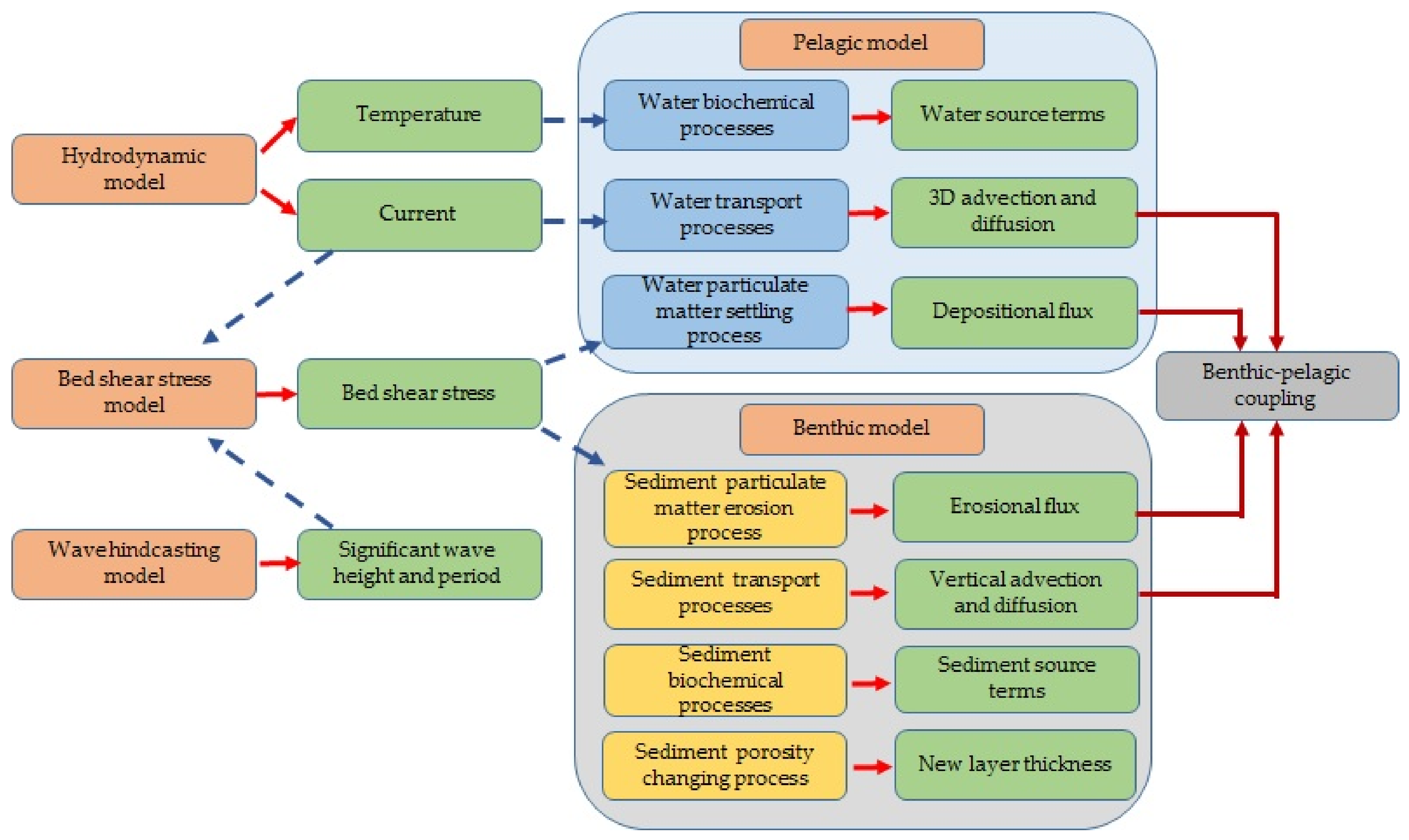
We first describe the integrated model framework and each of its constituents in detail. Then, we demonstrate its application to Tokyo Bay. The benthic–pelagic coupled, layer-resolved, and process-based 3D ecosystem model was integrated with 3D hydrodynamic [35], wave hindcasting [36], and bed shear stress (BSS) [5] models (Figure 2).

The hydrodynamic model computes the current field, which is applied for the computation of the water transport processes in the pelagic model and for the computation of CBSS in the BSS model. Moreover, it computes water temperature and salinity, which affect water and sediment quality. The WBSS is computed by using a significant wave height and wave period, which have been obtained from the wave hindcasting model. CBSS and WBSS are used in the model to compute the BSS, which is applied in particulate matter settling and sediment-resuspension process modeling.

2.1. Integrated Model Framework

Process-based coastal ecosystem models mainly consider physical processes, bioprocesses, and chemical processes. Other than those general processes, the mechanism of changing porosity with respect to POCC in sediment, which has emerged from the field data analysis [39], has been considered in this model. The processes in the water and sediment columns were considered independently, and the water column was coupled to the sediment column through the interaction of layer flux exchanges. Horizontal and vertical advection and diffusion processes were computed as water transport processes in the pelagic model, while only vertical advection and diffusion were computed as sediment transport processes in the benthic model. The particulate matter settling process was computed together with the sediment resuspension effects.

Phytoplankton and zooplankton processes were modeled as bio processes in the pelagic model, while benthic animals were not considered in the current model. The chemical processes of nutrients and aerobic and anaerobic decomposition of POC were computed for both the pelagic and benthic systems. Moreover, the process of porosity change with respect to POCC in sediment was modeled and it changed the concentrations of sediment variables at every time step owing to the change in layer thickness.

2.2. Hydrodynamic Model

A quasi-three-dimensional hydrodynamic model developed by [35] was applied. The model was governed by primitive equations with hydrostatic and Boussinesq approximations in $\sigma$-coordinates.

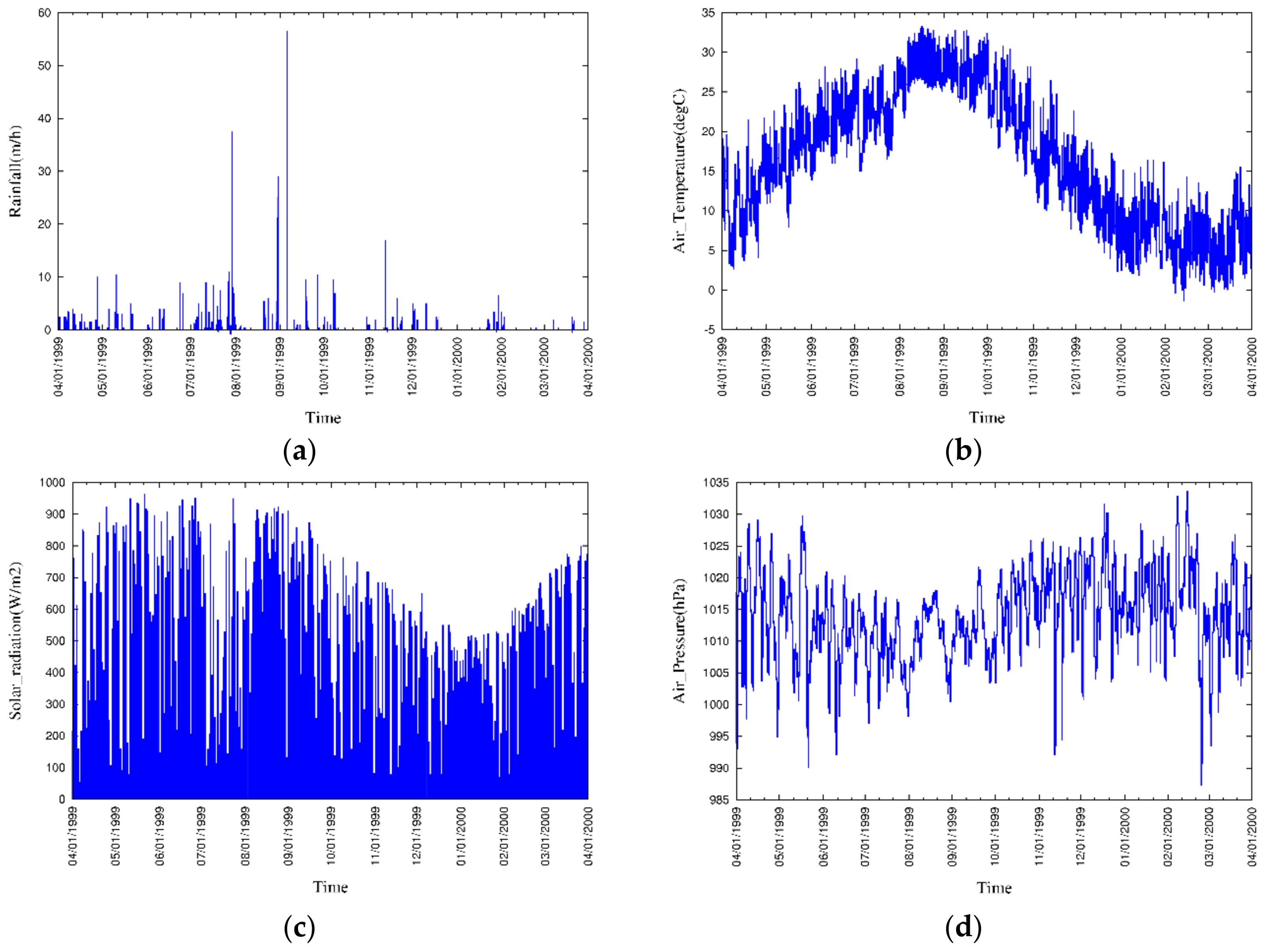
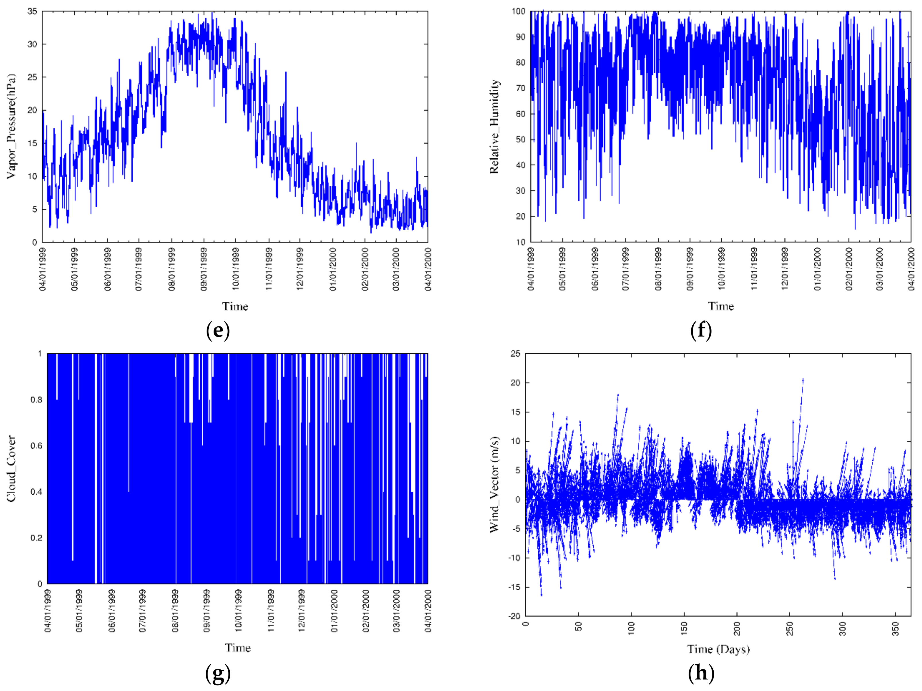
The model boundary conditions were considered at the bay mouth, free water surface, and bottom of the water column. At the bay mouth tidal level, water temperature and salinity were given. At the surface boundary, the model was forced by meteorological data, which includes rainfall, air temperature, solar radiation, air pressure, vapor pressure, relative humidity, cloud cover, wind vector, and instantaneous tidal motion. At the surface boundary, the pseudo velocity was set to zero, and the tangential stress at the free surface along the horizontal direction was made equal to the wind stress. At the sea bottom boundary, the pseudo velocity was set to zero, and the quadratic dependence of the bottom stress on the velocity has been considered. At lateral wall boundaries, normal velocities have been set to zero and free-slip conditions have been applied for the friction terms.

The governing equations were solved by a semi-implicit robust algorithm [35,44]. The water surface elevation, vertical advection, and vertical diffusion terms were discretized implicitly, while other terms were discretized explicitly. A staggered grid system was applied in the model control-volume face velocities were evaluated by the first-order upwind scheme and discretized equations were interpreted as a system of tri-diagonal matrixes and the tri-diagonal matrix algorithm (TDMA) [45] was applied to solve the system.

2.3. Wave Hindcasting Model

The wind-generated wave-hindcasting model developed by the Coastal Engineering Research Center [46] with the modifications proposed by [36] was adopted in this integrated modeling. This model has been developed for both shallow and deep waters through a set of parametric equations, which compute spatial and temporal variations in significant wave height and period.

The wave growth pattern has been considered as a combined characteristic of fetch and duration limited conditions. Under the fetch limited conditions, wind has to be blown constantly, long enough for wave heights at the end of the fetch to reach its equilibrium, while under duration limited conditions, the length of the time during which the wind has blown limits the wave height. The wave growth pattern in deep waters was obtained by simplifying the equations of the parametric model [47].

The wave growth pattern in shallow waters was based on approximations, in which the wave energy is increased owing to wind stress and reduced owing to bottom friction and percolation. Shallow water equations were the same as the expressions in [48,49,50] with a modified computation of fetch length. The fetch length was calculated as effective fetch, assuming that one fetch is computed as the summation of multi directional individual fetches [36]. This model has been validated by Rasmeemasmuang and Sasaki [5] and Achiari and Sasaki [36] for Tokyo Bay with the measured data, and Attari and Sasaki [40] has applied this model in their water quality modeling.

2.4. Bed Shear Stress (BSS) Model

The sediment dynamic process, including for instance sediment deposition and resuspension, is controlled by BSS in the bottom boundary layer. The BSS model proposed by Rasmeemasmuang and Sasaki [5] and applied by Attari and Sasaki [40] for Tokyo Bay has been integrated with this ecosystem model. The BSS has been estimated as a combined characteristic of wave and current motions. It has been assumed that this combined effect can be computed as a summation of the independent components of wave induced BSS (WBSS) and current induced BSS (CBSS) [51,52].

2.5. Pelagic Model

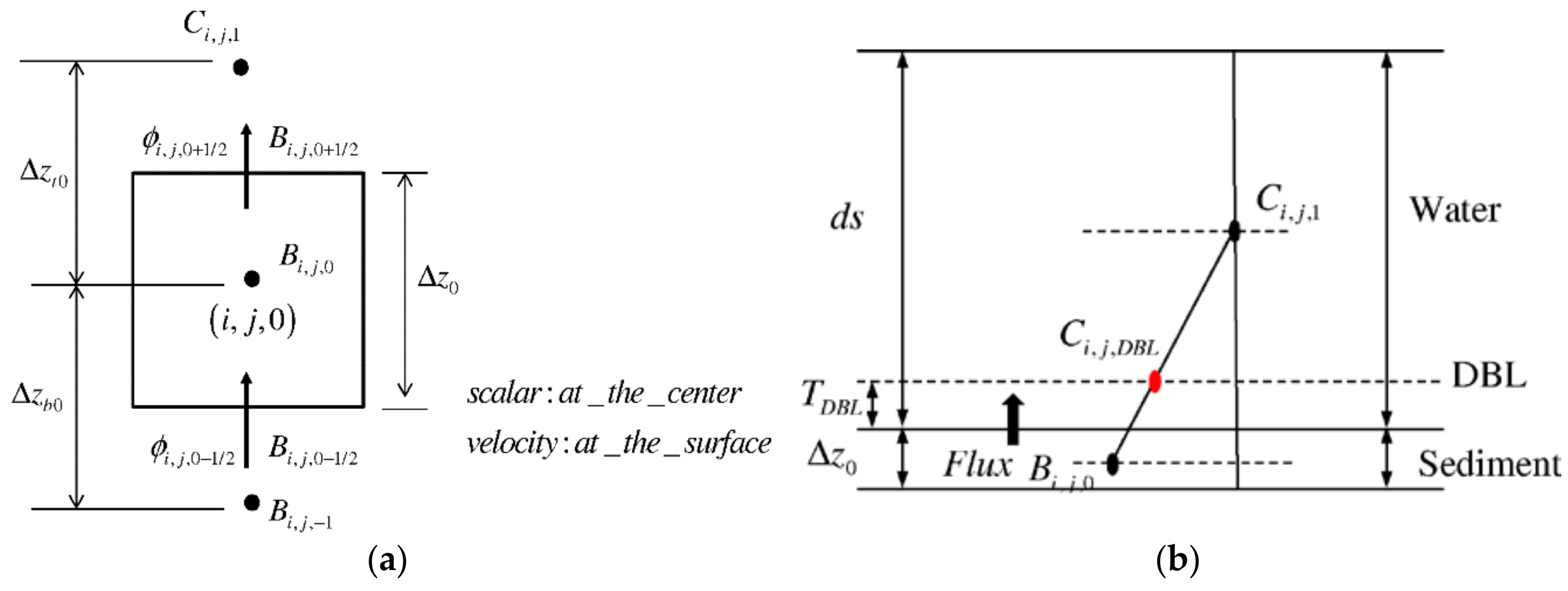
A 3D, layer-resolved water quality model was developed here. The main state variables for the model are three types of organic carbon, namely, labile, refractory, and inert; three types of phytoplankton, which have been categorized on seasonal blooms; zooplankton; dissolved oxygen (DO); nutrients such as ammonium-nitrogen, nitrate-nitrogen, and phosphate-phosphorus; two types of silica, namely, dissolved silica and particulate biogenic silica; sulfide; and suspended sediment. The pelagic model is composed of 20 $\sigma$-layers in vertical direction and uniformly structured grids in the horizontal space. The three dimensional layer resolved advection and diffusion equation in $\sigma$-coordinates for any scalar parameter in the water column by adopting control volume formulation

$$\frac{\partial (DC)}{\partial t}+\frac{\partial (uDC)}{\partial x}+\frac{\partial (vDC)}{\partial y}+\frac{\partial \left[(\dot{\sigma }+{\dot{\sigma }}_s)DC\right]}{\partial \sigma }=D{K}_h\left(\frac{{\partial }^{2}C}{\partial x^2}+\frac{{\partial }^{2}C}{\partial y^2}\right)+\frac{1}{D}\frac{\partial }{\partial \sigma }\left(K_v\frac{\partial C}{\partial \sigma }\right)+D{\displaystyle \sum _s{R}_s}$$

(1)

where $t$ is time, $(x,y,\sigma )$ are the sigma coordinates, $(u,v,\dot{\sigma })$ are the corresponding velocity components, $C$ is any state variable at any $(i,j,k)$ grid point, $R_s$ is the source term for the corresponding state variable, ${\dot{\sigma }}_s$ is the settling velocity in $\sigma$-coordinates given by ${\dot{\sigma }}_s=w_s/D$ [35] (this will be zero for dissolved matters) when $w_s$ is the settling velocity in Cartesian coordinates, and $D$ is the total depth. $K_h$ and $K_v$ are the horizontal and vertical kinematic eddy diffusivities, respectively.

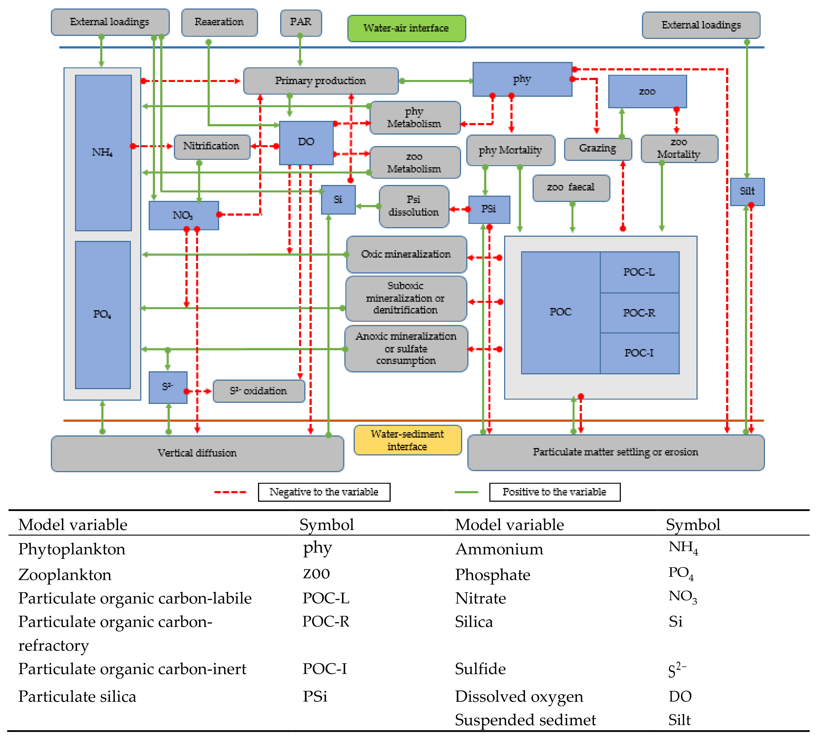
The biochemical processes, their interconnections with other variables, and, the benthic–pelagic coupling are shown in Figure 3. The main processes include the primary production that occurs when ammonium and nitrate are considered as electron accepters, phytoplankton metabolism and mortality, zooplankton grazing and mortality, mineralization under oxic, sub-oxic (denitrification), and anoxic (sulfur production) conditions, nitrification, oxidization of sulfide, and particulate silica dissolution. All the stoichiometric relationships associated with the biochemical processes are presented in

Table 1. Stoichiometric relationships associated with biochemical processes (modified from [6]).

Photosynthesis—ammonia as electron accepter ${106(\mathrm{CO}}_2{)+16(\mathrm{NH}}_3{)+\mathrm{H}}_3{\mathrm{PO}}_4{+106(\mathrm{H}}_2\mathrm{O})\to {{(\mathrm{CH}}_2\mathrm{O})}_{106}{{(\mathrm{NH}}_3)}_{16}{(\mathrm{H}}_3{\mathrm{PO}}_4{)+106(\mathrm{O}}_2)$

Photosynthesis—nitrate as electron accepter ${106(\mathrm{CO}}_2{)+16(\mathrm{NO}}_3^{-}{)+\mathrm{H}}_3{\mathrm{PO}}_4{+122(\mathrm{H}}_2{\mathrm{O})+16\mathrm{H}}^{+}\to {{(\mathrm{CH}}_2\mathrm{O})}_{106}{{(\mathrm{NH}}_3)}_{16}{(\mathrm{H}}_3{\mathrm{PO}}_4{)+138(\mathrm{O}}_2)$

Oxic mineralization and metabolism ${{(\mathrm{CH}}_2\mathrm{O})}_{106}{{(\mathrm{NH}}_3)}_{16}{(\mathrm{H}}_3{\mathrm{PO}}_4{)+106(\mathrm{O}}_2)\to {106(\mathrm{CO}}_2{)+16(\mathrm{NH}}_3{)+\mathrm{H}}_3{\mathrm{PO}}_4{+106(\mathrm{H}}_2\mathrm{O})$

Sub-oxic mineralization or denitrification ${{(\mathrm{CH}}_2\mathrm{O})}_{106}{{(\mathrm{NH}}_3)}_{16}{(\mathrm{H}}_3{\mathrm{PO}}_4)+\raisebox{1ex}{$424$}\!\left/ \!\raisebox{-1ex}{$5$}\right.{(\mathrm{HNO}}_3)\to {106(\mathrm{CO}}_2{)+16(\mathrm{NH}}_3{)+\mathrm{H}}_3{\mathrm{PO}}_4+\raisebox{1ex}{$106$}\!\left/ \!\raisebox{-1ex}{$5$}\right.{(\mathrm{H}}_2\mathrm{O})+\raisebox{1ex}{$212$}\!\left/ \!\raisebox{-1ex}{$5$}\right.{(\mathrm{N}}_2)$

Anoxic mineralization or H2S production ${{(\mathrm{CH}}_2\mathrm{O})}_{106}{{(\mathrm{NH}}_3)}_{16}{(\mathrm{H}}_3{\mathrm{PO}}_4)+\raisebox{1ex}{$106$}\!\left/ \!\raisebox{-1ex}{$2$}\right.{(\mathrm{H}}_2{\mathrm{SO}}_4)\to {106(\mathrm{CO}}_2{)+16(\mathrm{NH}}_3{)+\mathrm{H}}_3{\mathrm{PO}}_4{+106(\mathrm{H}}_2\mathrm{O})+\raisebox{1ex}{$106$}\!\left/ \!\raisebox{-1ex}{$2$}\right.{(\mathrm{H}}_2\mathrm{S})$

Nitrification ${\mathrm{NH}}_4^{+}{+2\mathrm{O}}_2\to {\mathrm{NO}}_3^{-}{+\mathrm{H}}_2{\mathrm{O}+2\mathrm{H}}^{+}$

H2S oxidization ${\mathrm{S}}^{2-}{+2(\mathrm{O}}_2)\to {{\mathrm{SO}}_4}^{2-}$

. Descriptions of the notations in the pelagic model equations are listed in

Table A1. Symbols in model equations.

Symbol		Unit	Description
[Water]	[Sediment]
$S$		$[\mathrm{psu}]$	Salinity
$T$		[°C]	Temperature
$C_{\mathrm{phy}}$		$[{\mathrm{mgC}/\mathrm{m}}^3]$	Phytoplankton concentration
$C_{\mathrm{zoo}}$		$[{\mathrm{mgC}/\mathrm{m}}^3]$	Zooplankton concentration
$C_{\mathrm{chl}}$		$[{\mathrm{mgC}/\mathrm{m}}^3]$	Chlorophyll a concentration
$C_{\mathrm{POC}}$	$B_{\mathrm{POC}}$	$[{\mathrm{mgC}/\mathrm{m}}^3]$	Particulate organic carbon concentration
$C_{{\mathrm{NH}}_4}$	$B_{{\mathrm{NH}}_4}$	${[\mathrm{mmol}/\mathrm{m}}^3]$	Ammonium nitrogen concentration
$C_{{\mathrm{PO}}_4}$	$B_{{\mathrm{PO}}_4}$	${[\mathrm{mmol}/\mathrm{m}}^3]$	Phosphate phosphorous concentration
$C_{{\mathrm{NO}}_3}$	$B_{{\mathrm{NO}}_3}$	${[\mathrm{mmol}/\mathrm{m}}^3]$	Nitrate nitrogen concentration
$C_{\mathrm{Si}}$	$B_{\mathrm{Si}}$	${[\mathrm{mmol}/\mathrm{m}}^3]$	Dissolved silica concentration
$C_{\mathrm{PSi}}$	$B_{\mathrm{PSi}}$	${[\mathrm{mg}/\mathrm{m}}^3]$	Particulate biogenic silica concentration
$C_{\mathrm{DO}}$	$B_{\mathrm{DO}}$	${[\mathrm{g}/\mathrm{m}}^3]$	Dissolved oxygen concentration
$C_{{\mathrm{S}}^{2-}}$	$B_{{\mathrm{S}}^{2-}}$	${[\mathrm{g}/\mathrm{m}}^3]$	Sulfide concentration
$C_{\mathrm{Silt}}$	$B_{\mathrm{Silt}}$	${[\mathrm{g}/\mathrm{m}}^3]$	Silt concentration
Pelagic model
[Phytoplankton model]
$R_{\mathrm{phy}\_\mathrm{PP}}$		${[\mathrm{mgC}/\mathrm{m}}^3/\mathrm{s}]$	Rate of primary production
$R_{\mathrm{phy}\_\mathrm{Met}}$		${[\mathrm{mgC}/\mathrm{m}}^3/\mathrm{s}]$	Rate of metabolism
$R_{\mathrm{phy}\_\mathrm{Mor}}$		${[\mathrm{mgC}/\mathrm{m}}^3/\mathrm{s}]$	Rate of mortality
$R_{\mathrm{zoo}\_\mathrm{GE}}$		${[\mathrm{mgC}/\mathrm{m}}^3/\mathrm{s}]$	Rate of zooplankton grazing on each food
$G_{\mathrm{phy}}$		[1/s]	Maximum rate of phytoplankton growth at 20 °C
$M_{\mathrm{phy}}$		[1/s]	Maximum rate of phytoplankton metabolism at 20 °C
$D_{\mathrm{phy}}$		[1/s]	Maximum rate of phytoplankton mortality at 20 °C
$f_{\mathrm{TLphy}}$		-	Temperature limit for phytoplankton growth
$f_{\mathrm{LLphy}}$		-	Light limit for phytoplankton growth
$f_{\mathrm{NLphy}}$		-	Nutrient limit for phytoplankton growth
${\mathrm{PO}}_{4\mathrm{NLphy}}$		-	Phosphate nutrient limit for phytoplankton growth
${\mathrm{nit}}_{\mathrm{NLphy}}$		-	Nitrogen nutrient limit for phytoplankton growth
${\mathrm{Si}}_{\mathrm{NLphy}}$		-	Silica nutrient limit for phytoplankton growth
$T_{\mathrm{LO}}$		[°C]	Lower end of optimal temperature
$T_{\mathrm{UO}}$		[°C]	Upper end of optimal temperature
$K_{{\mathrm{PO}}_4}$		${[\mathrm{mmol}/\mathrm{m}}^3]$	Half saturation constant of phosphorous limitation
$K_{\mathrm{nit}}$		${[\mathrm{mmol}/\mathrm{m}}^3]$	Half saturation constant of nitrogen limitation
$K_{\mathrm{Si}}$		${[\mathrm{mmol}/\mathrm{m}}^3]$	Half saturation constant of silica limitation
$\mathrm{PAR}$		${[\mathrm{J}/\mathrm{m}}^2/\mathrm{s}]$	Photosynthetically active radiation
${\mathrm{PAR}}_{\mathrm{sur}}$		${[\mathrm{J}/\mathrm{m}}^2/\mathrm{s}]$	Photosynthetically active radiation at surface
${\mathrm{PAR}}_{\mathrm{opt}}$		${[\mathrm{J}/\mathrm{m}}^2/\mathrm{s}]$	Optimum of photosynthetically active radiation
${\mathrm{PAR}}_{\min }$		${[\mathrm{J}/\mathrm{m}}^2/\mathrm{s}]$	Minimum of photosynthetically active radiation
$k_e$		-	Light extinction coefficient
[Zooplankton model]
$R_{\mathrm{zoo}\_\mathrm{Gro}}$		${[\mathrm{mgC}/\mathrm{m}}^3/\mathrm{s}]$	Rate of zooplankton growth
$R_{\mathrm{zoo}\_\mathrm{Mor}}$		${[\mathrm{mgC}/\mathrm{m}}^3/\mathrm{s}]$	Rate of zooplankton mortality
$R_{\mathrm{zoo}\_\mathrm{A}}$		${[\mathrm{mgC}/\mathrm{m}}^3/\mathrm{s}]$	Rate of zooplankton absorption
$R_{\mathrm{zoo}\_\mathrm{MF}}$		${[\mathrm{mgC}/\mathrm{m}}^3/\mathrm{s}]$	Rate of availability of minimum food for zooplankton
$R_{\mathrm{MAX}\_\mathrm{MF}}$		[1/s]	Maximum rate of minimum food for zooplankton at 20 °C
$C_{\mathrm{zoo}\_\mathrm{AP}}$		-	Maximum absorb portion of food by zooplankton at 20 °C
$K_{\mathrm{DO}\_\mathrm{zoo}}$		${[\mathrm{gO}}_2{/\mathrm{m}}^3]$	Oxygen half saturation constant for zooplankton metabolism
$R_{\mathrm{zoo}\_\mathrm{G}}$		${[\mathrm{mgC}/\mathrm{m}}^3/\mathrm{s}]$	Rate of zooplankton grazing at 20 °C
$R_{\mathrm{zoo}\_\mathrm{GE}}$		${[\mathrm{mgC}/\mathrm{m}}^3/\mathrm{s}]$	Rate of zooplankton grazing for each food at 20 °C
$R_{\mathrm{zoo}\_\mathrm{GP}}$		${[\mathrm{mgC}/\mathrm{m}}^3/\mathrm{s}]$	Grazing primitive of zooplankton
$G_{\mathrm{zoo}}$		[1/s]	Maximum rate of zooplankton growth at 20 °C
$f_{\mathrm{TLzoo}}$		-	Temperature limit for zooplankton
$f_{\mathrm{FLzoo}}$		-	Food limit for zooplankton
$\mathrm{Food}\_\mathrm{Thr}$		$[{\mathrm{mgC}/\mathrm{m}}^3]$	Threshold food concentration
$K_{\mathrm{Ivlev}}$		$[{\mathrm{m}}^3/\mathrm{mgC}]$	Total food proportionality constant for Ivlev formulation
$R_{\mathrm{zoo}\_\mathrm{Fecal}}$		$[{\mathrm{mgC}/\mathrm{m}}^3/\mathrm{s}]$	Rate of zooplankton fecal at 20 °C
$C_{\mathrm{zoo}\_\mathrm{MAX}}$		$[{\mathrm{mgC}/\mathrm{m}}^3]$	Maximum concentration of zooplankton at 20 °C
$D_{\mathrm{zoo}}$		[1/s]	Maximum rate of zooplankton mortality at 20 °C
[Particulate organic carbon model]
$R_{C_{\mathrm{POC}}\_\mathrm{O}}$		${[\mathrm{mgC}/\mathrm{m}}^3/\mathrm{s}]$	Rate of aerobic decomposition
$k_{C_{\mathrm{POC}}\_\mathrm{O}}$		[1/s]	Maximum rate of aerobic decomposition at 20 °C
${\theta }_{C_{\mathrm{POC}}}$		-	Temperature coefficient for aerobic decomposition
$K_{\mathrm{DO},C_{\mathrm{POC}}}$		${[\mathrm{gO}}_2{/\mathrm{m}}^3]$	Oxygen half saturation constant for aerobic decomposition
$R_{C_{\mathrm{POC}}\_{\mathrm{NO}}_3}$		${[\mathrm{mgC}/\mathrm{m}}^3/\mathrm{s}]$	Rate of denitrification as a fraction of POC
$R_{C_{{\mathrm{NO}}_3}\_D}$		${[\mathrm{mgC}/\mathrm{m}}^3/\mathrm{s}]$	Rate of denitrification
$k_{C_{{\mathrm{NO}}_3}\_D}$		[1/s]	Maximum rate of denitrification at 20 °C
${\theta }_{C_{{\mathrm{NO}}_3}}$		-	Temperature coefficient for denitrification
$K_{\mathrm{dec},C_{\mathrm{POC}}}$		${[\mathrm{mgC}/\mathrm{m}}^3]$	Half saturation constant for POC in denitrification
$R_{C_{\mathrm{POC}}\_{\mathrm{SO}}_4}$		${[\mathrm{mgC}/\mathrm{m}}^3/\mathrm{s}]$	Rate of anaerobic decomposition
$k_{C_{\mathrm{POC}}\_{\mathrm{SO}}_4}$		[1/s]	Maximum rate of anaerobic decomposition at 20 °C
${\theta }_{C_{\mathrm{POC}}\_{\mathrm{SO}}_4}$		-	Temperature coefficient for anaerobic decomposition
$K_{C_{{\mathrm{NO}}_3}\_D}$		${[\mathrm{mmol}/\mathrm{m}}^3]$	Half saturation constant for denitrification
$F$		-	Fraction of particulate organic carbon
[Ammonia model]
$R_{C_{{\mathrm{NH}}_4}\_\mathrm{N}}$		${[\mathrm{mmol}/\mathrm{m}}^3/\mathrm{s}]$	Rate of nitrification
$k_{C_{{\mathrm{NH}}_4}\_\mathrm{N}}$		[1/s]	Maximum rate of nitrification at 20 °C
${\theta }_{C_{{\mathrm{NH}}_4}\_\mathrm{N}}$		-	Temperature coefficient for nitrification
$K_{\mathrm{DO},C_{{\mathrm{NH}}_4}}$		${[\mathrm{gO}}_2{/\mathrm{m}}^3]$	Oxygen half saturation constant for nitrification
[Silica model]
$R_{C_{\mathrm{Si}}\_\mathrm{Pro}}$		${[\mathrm{mmol}/\mathrm{m}}^3/\mathrm{s}]$	Rate of silica production
$k_{C_{\mathrm{Si}}}$		[1/s]	Maximum rate of silica production at 20 °C
${\theta }_{C_{\mathrm{Si}}}$		-	Temperature coefficient for particulate silica dissolution
$K_{C_{\mathrm{PSi}}}$		${[\mathrm{mmol}/\mathrm{m}}^3]$	Half saturation constant for particulate silica dissolution
$C_{\mathrm{Si},\mathrm{sat}}$		${[\mathrm{mmol}/\mathrm{m}}^3]$	Saturated concentration of silica
[Sulfide model]
$R_{C_{S^{2-}}\_\mathrm{O}}$		${[\mathrm{gS}/\mathrm{m}}^3/\mathrm{s}]$	Rate of sulfide oxidization
$k_{C_{S^{2-}}\_\mathrm{O}}$		[1/s]	Maximum rate of sulfide oxidization at 20 °C
${\theta }_{C_{S^{2-}}}$		-	Temperature coefficient for sulfide oxidization
$K_{\mathrm{DO},C_{S^{2-}}}$		${[\mathrm{gS}/\mathrm{m}}^3]$	Oxygen half saturation constant for sulfide oxidation
Benthic model
[Particulate organic carbon model]
$R_{B_{\mathrm{POC}}\_\mathrm{O}}$		${[\mathrm{mgC}/\mathrm{m}}^3/\mathrm{s}]$	Rate of aerobic decomposition
$k_{B_{\mathrm{POC}}\_\mathrm{O}}$		[1/s]	Maximum rate of aerobic decomposition at 20 °C
${\theta }_{B_{\mathrm{POC}}}$		-	Temperature coefficient for aerobic decomposition
$K_{\mathrm{DO},B_{\mathrm{POC}}}$		${[\mathrm{gO}}_2{/\mathrm{m}}^3]$	Oxygen half saturation constant for aerobic decomposition
$R_{B_{\mathrm{POC}}\_{\mathrm{NO}}_3}$		${[\mathrm{mgC}/\mathrm{m}}^3/\mathrm{s}]$	Rate of denitrification as a fraction of POC
$R_{B_{{\mathrm{NO}}_3}\_D}$		${[\mathrm{mgC}/\mathrm{m}}^3/\mathrm{s}]$	Rate of denitrification
$k_{B_{{\mathrm{NO}}_3}\_D}$		[1/s]	Maximum rate of denitrification at 20 °C
${\theta }_{B_{{\mathrm{NO}}_3}}$		-	Temperature coefficient for denitrification
$K_{\mathrm{dec},B_{\mathrm{POC}}}$		${[\mathrm{mgC}/\mathrm{m}}^3]$	Half saturation constant for POC in denitrification
$R_{B_{\mathrm{POC}}\_{\mathrm{SO}}_4}$		${[\mathrm{mgC}/\mathrm{m}}^3/\mathrm{s}]$	Rate of anaerobic decomposition
$k_{B_{\mathrm{POC}}\_{\mathrm{SO}}_4}$		[1/s]	Maximum rate of anaerobic decomposition at 20 °C
${\theta }_{B_{\mathrm{POC}}\_{\mathrm{SO}}_4}$		-	Temperature coefficient for anaerobic decomposition
$K_{B_{{\mathrm{NO}}_3}\_D}$		${[\mathrm{mmol}/\mathrm{m}}^3]$	Half saturation constant for denitrification
[Ammonia model]
$R_{B_{{\mathrm{NH}}_4}\_\mathrm{N}}$		${[\mathrm{mmol}/\mathrm{m}}^3/\mathrm{s}]$	Rate of nitrification
$k_{B_{{\mathrm{NH}}_4}\_\mathrm{N}}$		[1/s]	Maximum rate of nitrification at 20 °C
${\theta }_{B_{{\mathrm{NH}}_4}\_\mathrm{N}}$		-	Temperature coefficient for nitrification
$K_{\mathrm{DO},B_{{\mathrm{NH}}_4}}$		${[\mathrm{gO}}_2{/\mathrm{m}}^3]$	Oxygen half saturation constant for nitrification
[Silica model]
$R_{B_{\mathrm{Si}}\_\mathrm{Pro}}$		${[\mathrm{mmol}/\mathrm{m}}^3/\mathrm{s}]$	Rate of silica production
$k_{B_{\mathrm{Si}}}$		[1/s]	Maximum rate of silica production at 20 °C
${\theta }_{B_{\mathrm{Si}}}$		-	Temperature coefficient for particulate silica dissolution
$K_{B_{\mathrm{PSi}}}$		${[\mathrm{mmol}/\mathrm{m}}^3]$	Half saturation constant for particulate silica dissolution
$B_{\mathrm{Si},\mathrm{sat}}$		${[\mathrm{mmol}/\mathrm{m}}^3]$	Saturated concentration of silica
[Sulfide model]
$R_{B_{S^{2-}}\_\mathrm{O}}$		${[\mathrm{gS}/\mathrm{m}}^3/\mathrm{s}]$	Rate of sulfide oxidization
$k_{B_{S^{2-}}\_\mathrm{O}}$		[1/s]	Maximum rate of sulfide oxidization at 20 °C
${\theta }_{B_{S^{2-}}}$		-	Temperature coefficient for sulfide oxidization
$K_{\mathrm{DO},B_{S^{2-}}}$		${[\mathrm{gS}/\mathrm{m}}^3]$	Half saturation constant of oxygen for sulfide oxidization
[Transfer ratios]
$r_{\mathrm{PC}\_\mathrm{dec}}$		$[\mathrm{mmolP}/\mathrm{mgC}]$	Ratio of phosphorous to carbon for particulate organic carbon decomposition
$r_{\mathrm{NC}\_\mathrm{dec}}$		$[\mathrm{mmolN}/\mathrm{mgC}]$	Ratio of nitrogen to carbon for particulate organic carbon decomposition
$r_{\mathrm{CN}\_\mathrm{D}}$		$[\mathrm{mgC}/\mathrm{mmolN}]$	Ratio of carbon to nitrogen for denitrification
$r_{\mathrm{SiC}\_\mathrm{phy}}$		$[\mathrm{mmolSi}/\mathrm{mgC}]$	Ratio of silica to carbon for particulate organic carbon decomposition
$r_{\mathrm{Si}\_\mathrm{PSi}}$		$[\mathrm{mgSi}/\mathrm{mmolSi}]$	Ratio of dissolved silica to particulate silica
$r_{\mathrm{CS}\_\mathrm{dec}}$		$[\mathrm{gS}/\mathrm{mgC}]$	Ratio of carbon to sulfur for particulate organic carbon anoxic decomposition
$r_{\mathrm{OC}\_\mathrm{dec}}$		${[\mathrm{gO}}_2/\mathrm{mgC}]$	Ratio of oxygen to carbon for particulate organic carbon decomposition
$r_{\mathrm{ON}\_\mathrm{nit}}$		${[\mathrm{gO}}_2/\mathrm{mmolN}]$	Ratio of oxygen to nitrogen for nitrification
$r_{\mathrm{OS}\_\mathrm{oxi}}$		${[\mathrm{gO}}_2/\mathrm{gS}]$	Ratio of oxygen to sulfur for sulfide oxidization
Benthic–pelagic interaction parameters
${\mathrm{F}}_{{\mathrm{PO}}_4}$		${[\mathrm{mmol}/\mathrm{m}}^2/\mathrm{s}]$	Diffusion flux of phosphate between sediment and water
${\mathrm{F}}_{{\mathrm{NH}}_4}$		${[\mathrm{mmol}/\mathrm{m}}^2/\mathrm{s}]$	Diffusion flux of ammonia between sediment and water
${\mathrm{F}}_{{\mathrm{NO}}_3}$		${[\mathrm{mmol}/\mathrm{m}}^2/\mathrm{s}]$	Diffusion flux of nitrate between sediment and water
${\mathrm{F}}_{\mathrm{Si}}$		${[\mathrm{mmol}/\mathrm{m}}^2/\mathrm{s}]$	Diffusion flux of Silica between sediment and water
${\mathrm{F}}_{{\mathrm{S}}^{2-}}$		${[\mathrm{gS}/\mathrm{m}}^2/\mathrm{s}]$	Diffusion flux of sulfide between sediment and water
${\mathrm{F}}_{\mathrm{DO}}$		${[\mathrm{gO}}_2{/\mathrm{m}}^2/\mathrm{s}]$	Diffusion flux of oxygen between sediment and water

, and the model parameters for Tokyo Bay are listed in

Table A2. Model parameters.

Parameter	Units	Value	Main Source
Pelagic model
Phytoplankton model
$G_{\mathrm{phy}}$	[1/d]	(2.772, 2.772, 2.772) a	[6,75,76]
$M_{\mathrm{phy}}$	[1/d]	(0.083, 0.083, 0.083) a	[6,56,76]
$D_{\mathrm{phy}}$	[1/d]	(0.1386, 0.1386, 0.1386) a	[6,56,76]
$k_{\mathrm{GKL}}$	-	(0.8, 0.8, 0.8) a	[20]
$k_{\mathrm{GKU}}$	-	(0.8, 0.8, 0.8) a	[20]
$K_{{\mathrm{PO}}_4}$	${[\mathrm{mmol}/\mathrm{m}}^3]$	(1 × 10−8, 0.01, 1 × 10−3) a	[6,56,76]
$K_{\mathrm{nit}}$	${[\mathrm{mmol}/\mathrm{m}}^3]$	(0.5, 0.25, 1 × 10-3) a	[6,56,76]
$K_{\mathrm{Si}}$	${[\mathrm{mmol}/\mathrm{m}}^3]$	(1 × 10−3, 0.02, 1 × 10−3) a	[77]
${\mathrm{PAR}}_{\min }$	${[\mathrm{J}/\mathrm{m}}^2/\mathrm{s}]$	(2, 25, 25) a	Tuc
Zooplankton model
$R_{\mathrm{MAX}\_\mathrm{MF}}$	[1/d]	0.04	[78]
$C_{\mathrm{zoo}\_\mathrm{AP}}$	-	0.6	[76,78,79]
$K_{\mathrm{DO}\_\mathrm{zoo}}$	${[\mathrm{gO}}_2{/\mathrm{m}}^3]$	1.0	[78]
$G_{\mathrm{zoo}}$	[1/d]	0.2	[6,56,78]
$\mathrm{Food}\_\mathrm{Thr}$	$[{\mathrm{mgC}/\mathrm{m}}^3]$	0.01	[76,78,79]
$K_{\mathrm{Ivlev}}$	$[{\mathrm{m}}^3/\mathrm{mgC}]$	50.0	[78]
$C_{\mathrm{zoo}\_\mathrm{MAX}}$	$[{\mathrm{mgC}/\mathrm{m}}^3]$	100.0	Tuc
$D_{\mathrm{zoo}}$	[1/d]	0.05	[78]
Particulate organic carbon model
$k_{C_{\mathrm{POC}}\_\mathrm{O}}$	[1/d]	(0.35, 0.018, 0.0) b	[19]
${\theta }_{C_{\mathrm{POC}}}$	-	(1.08, 1.08, -) b	[19]
$K_{\mathrm{DO},C_{\mathrm{POC}}}$	${[\mathrm{gO}}_2{/\mathrm{m}}^3]$	0.1	[6]
$k_{C_{{\mathrm{NO}}_3}\_D}$	[1/d]	(2.0, 0.1, 0.0) b	Tuc
${\theta }_{C_{{\mathrm{NO}}_3}}$	-	1.086	[19]
$K_{\mathrm{dec},C_{\mathrm{POC}}}$	${[\mathrm{mgC}/\mathrm{m}}^3]$	10.0	Tuc
$k_{C_{\mathrm{POC}}\_{\mathrm{SO}}_4}$	[1/d]	(0.035, 0.0018, 0.0) b	[19]
${\theta }_{C_{\mathrm{POC}}\_{\mathrm{SO}}_4}$	-	(1.08, 1.15, -) b	[19]
$K_{C_{{\mathrm{NO}}_3}\_D}$	${[\mathrm{mmol}/\mathrm{m}}^3]$	0.5	[19]
$F$	-	(0.65, 0.25, 0.1) b	[19]
Ammonium model
$k_{C_{{\mathrm{NH}}_4}\_\mathrm{N}}$	[1/d]	0.06	Tuc
${\theta }_{C_{{\mathrm{NH}}_4}\_\mathrm{N}}$	-	1.123	[19]
$K_{\mathrm{DO},C_{{\mathrm{NH}}_4}}$	${[\mathrm{gO}}_2{/\mathrm{m}}^3]$	0.37	[19]
Silica model
$k_{C_{\mathrm{Si}}}$	[1/d]	1.925 × 10−3	[19]
${\theta }_{C_{\mathrm{Si}}}$	-	1.059	[19]
$K_{C_{\mathrm{PSi}}}$	$[\mathrm{mgSi}/\mathrm{l}]$	19.8	[19]
$C_{\mathrm{Si},\mathrm{sat}}$	$[\mathrm{mgSi}/\mathrm{l}]$	26.5	[19]
Sulfide model
$k_{C_{S^{2-}}\_\mathrm{O}}$	[1/d]	6.0	Tuc
${\theta }_{C_{S^{2-}}}$	-	1.123	[19]
$K_{\mathrm{DO},C_{S^{2-}}}$	${[\mathrm{gS}/\mathrm{m}}^3]$	2.0	[19]
Benthic model
Particulate organic carbon model
$k_{B_{\mathrm{POC}}\_\mathrm{O}}$	[1/d]	(0.35, 0.018, 0.0) b	[19]
${\theta }_{B_{\mathrm{POC}}}$	-	(1.08, 1.08, -) b	[19]
$K_{\mathrm{DO},B_{\mathrm{POC}}}$	${[\mathrm{gO}}_2{/\mathrm{m}}^3]$	0.1	[6]
$k_{B_{{\mathrm{NO}}_3}\_D}$	[1/d]	(2.0, 0.1, 0.0) b	Tuc
${\theta }_{B_{{\mathrm{NO}}_3}}$	-	1.086	[19]
$K_{\mathrm{dec},B_{\mathrm{POC}}}$	${[\mathrm{mgC}/\mathrm{m}}^3]$	5000.0	Tuc
$k_{B_{\mathrm{POC}}\_{\mathrm{SO}}_4}$	[1/d]	(0.035, 0.0018, 0.0) b	[19]
${\theta }_{B_{\mathrm{POC}}\_{\mathrm{SO}}_4}$	-	(1.08, 1.15, -) b	[19]
$K_{B_{{\mathrm{NO}}_3}\_D}$	${[\mathrm{mmol}/\mathrm{m}}^3]$	0.5	[19]
Ammonium model
$k_{B_{{\mathrm{NH}}_4}\_\mathrm{N}}$	[1/d]	140.63	Tuc
${\theta }_{B_{{\mathrm{NH}}_4}\_\mathrm{N}}$	-	1.123	[19]
$K_{\mathrm{DO},B_{{\mathrm{NH}}_4}}$	${[\mathrm{gO}}_2{/\mathrm{m}}^3]$	0.37	[19]
Silica model
$k_{B_{\mathrm{Si}}}$	[1/d]	1.925 × 10−3	[19]
${\theta }_{B_{\mathrm{Si}}}$	-	1.059	[19]
$K_{B_{\mathrm{PSi}}}$	$[\mathrm{mgSi}/\mathrm{l}]$	19.8	[19]
$B_{\mathrm{Si},\mathrm{sat}}$	$[\mathrm{mgSi}/\mathrm{l}]$	26.5	[19]
Sulfide model
$k_{B_{S^{2-}}\_\mathrm{O}}$	[1/d]	6.0	Tuc
${\theta }_{B_{S^{2-}}}$	-	1.123	[19]
$K_{\mathrm{DO},B_{S^{2-}}}$	${[\mathrm{gS}/\mathrm{m}}^3]$	0.0001	[19]
Transfer ratios
$r_{\mathrm{PC}\_\mathrm{dec}}$	$[\mathrm{mmolP}/\mathrm{mgC}]$	1.0/(12.0 × 106.0)	[19]
$r_{\mathrm{NC}\_\mathrm{dec}}$	$[\mathrm{mmolN}/\mathrm{mgC}]$	16.0/(12.0 × 106.0)	[19]
$r_{\mathrm{CN}\_\mathrm{D}}$	$[\mathrm{mgC}/\mathrm{mmolN}]$	(106.0 × 12.0 × 5.0)/424.0	[18,19]
$r_{\mathrm{SiC}\_\mathrm{phy}}$	$[\mathrm{mmolSi}/\mathrm{mgC}]$	1.0/(12.0 × 8.0)	[19]
$r_{\mathrm{Si}\_\mathrm{PSi}}$	$[\mathrm{mgSi}/\mathrm{mmolSi}]$	28.0	[19]
$r_{\mathrm{CS}\_\mathrm{dec}}$	$[\mathrm{gS}/\mathrm{mgC}]$	(53.0 × 32.0 × 10−3)/(106.0 × 12.0)	[18,19]
$r_{\mathrm{OC}\_\mathrm{dec}}$	${[\mathrm{gO}}_2/\mathrm{mgC}]$	(32.0 × 10−3)/12.0	[19]
$r_{\mathrm{ON}\_\mathrm{nit}}$	${[\mathrm{gO}}_2/\mathrm{mmolN}]$	4.33 × 14.0 × 10−3	[18,19]
$r_{\mathrm{OS}\_\mathrm{oxi}}$	${[\mathrm{gO}}_2/\mathrm{gS}]$	2.0	[19]

^a—values for three groups of phytoplankton, ^b—values for three groups of POC (POC-L, POC-R, and POC-I). Tu^c—tuning parameter.

. The expressions for the biochemical kinetic processes basically followed the formulae adopted in conventional models [19,20] (

Table A3. Kinetic equations for source terms in pelagic model (see Appendix A (Table A1) for symbols).

Biochemical Process	Formulation
Phytoplankton	$\frac{d{C}_{\mathrm{phy}}}{dt}=\left[\begin{array}{l}\mathrm{Primary}\_\mathrm{Production}-{\mathrm{Metabolism}}_{\mathrm{phy}}-{\mathrm{Mortality}}_{\mathrm{phy}}\\ -\mathrm{Zoo}\_\mathrm{Grazing}\end{array}\right]$ $\frac{d{C}_{\mathrm{phy}}}{dt}=\left[R_{\mathrm{phy}\_\mathrm{PP}}-R_{\mathrm{phy}\_\mathrm{Met}}-R_{\mathrm{phy}\_\mathrm{Mor}}-R_{\mathrm{zoo}\_\mathrm{GE}}\right]$
Primary production:	$R_{\mathrm{phy}\_\mathrm{PP}}=G_{\mathrm{phy}}{f}_{\mathrm{TLphy}}{f}_{\mathrm{LLphy}}{f}_{\mathrm{NLphy}}{C}_{\mathrm{phy}}$
	$f_{\mathrm{TLphy}}=\left\{\begin{array}{cc}\exp \{-k_{\mathrm{GKL}}{(T-T_{\mathrm{LO}})}^2\}\hfill & (T<T_{\mathrm{LO}})\\ 1\hfill & (T_{\mathrm{LO}}<T<T_{\mathrm{UO}})\\ \exp \{-k_{\mathrm{GKU}}{(T-T_{\mathrm{UO}})}^2\}\hfill & (T>T_{\mathrm{UO}})\end{array}\right\}$
	$f_{\mathrm{LLphy}}=\frac{\mathrm{PAR}}{{\mathrm{PAR}}_{\mathrm{opt}}}\exp \left\{1-\frac{\mathrm{PAR}}{{\mathrm{PAR}}_{\mathrm{opt}}}\right\}$
	$\mathrm{PAR}={\mathrm{PAR}}_{\mathrm{sur}}\exp \{-k_{\mathrm{e}}\mathrm{D}\}$
	$k_{\mathrm{e}}=0.32+0.016C_{\mathrm{chl}}+0.094C_{\mathrm{Silt}}$
	${\mathrm{PAR}}_{\mathrm{opt}}=\mathrm{MAX}\left(\frac{\mathrm{PAR}}{\mathrm{PI}},{\mathrm{PAR}}_{\min }\right)$
	$f_{\mathrm{NLphy}}=\mathrm{MIN}\left({\mathrm{PO}}_{4\mathrm{NLphy}},{\mathrm{nit}}_{\mathrm{NLphy}},{\mathrm{Si}}_{\mathrm{NLphy}}\right)$
	${\mathrm{PO}}_{4\mathrm{NLphy}}=f_{\mathrm{Monod}}(C_{{\mathrm{PO}}_4},K_{{\mathrm{PO}}_4})$
	${\mathrm{nit}}_{\mathrm{NLphy}}=f_{\mathrm{Monod}}(C_{{\mathrm{NH}}_4}+C_{{\mathrm{NO}}_3},K_{\mathrm{nit}})$
	${\mathrm{Si}}_{\mathrm{NLphy}}=f_{\mathrm{Monod}}(C_{\mathrm{Si}},K_{\mathrm{Si}})$
	$f_{\mathrm{Monod}}(\mathrm{Nut},\mathrm{Hf}\_\mathrm{Nut})=\frac{\mathrm{Nut}}{\mathrm{Hf}\_\mathrm{Nut}+\mathrm{Nut}}$
Metabolism:	$R_{\mathrm{phy}\_\mathrm{Met}}=M_{\mathrm{phy}}\exp (0.04(T-20))C_{\mathrm{phy}}$
Mortality:	$R_{\mathrm{phy}\_\mathrm{Mor}}=D_{\mathrm{phy}}{C}_{\mathrm{phy}}$
Zooplankton Grazing:	$R_{zoo\_\mathrm{GE}}=\mathrm{From}\mathrm{zooplankton}\mathrm{model}$
Zooplankton	$\frac{d{C}_{\mathrm{zoo}}}{dt}=\left[\mathrm{Growth}-{\mathrm{Mortality}}_{zoo}\right]$ $\frac{d{C}_{\mathrm{zoo}}}{dt}=\left[R_{\mathrm{zoo}\_\mathrm{Gro}}-R_{\mathrm{zoo}\_\mathrm{Mor}}\right]$
Growth:	$R_{\mathrm{zoo}\_\mathrm{Gro}}=R_{\mathrm{zoo}\_\mathrm{A}}-R_{\mathrm{zoo}\_\mathrm{MF}}$
	$R_{\mathrm{zoo}\_\mathrm{A}}=C_{\mathrm{zoo}\_\mathrm{AP}}{R}_{\mathrm{zoo}\_\mathrm{G}}{f}_{\mathrm{Monod}}(C_{\mathrm{DO}},K_{\mathrm{DO}\_\mathrm{zoo}})$
	$R_{\mathrm{zoo}\_\mathrm{G}}={\displaystyle \sum _{\mathrm{F}\_\mathrm{iter}=1}^{\mathrm{p}}{R}_{\mathrm{zoo}\_\mathrm{GE}}(\mathrm{F}\_\mathrm{iter})}$
	$R_{\mathrm{zoo}\_\mathrm{GE}}(\mathrm{F}\_\mathrm{iter})=R_{\mathrm{zoo}\_\mathrm{GP}}\frac{\mathrm{F}\_\mathrm{each}(\mathrm{F}\_\mathrm{iter})}{\mathrm{Total}\_\mathrm{F}}$
	$R_{\mathrm{zoo}\_\mathrm{GP}}=G_{\mathrm{zoo}}{f}_{\mathrm{TLzoo}}{f}_{\mathrm{FLzoo}}{C}_{\mathrm{zoo}}$
	$f_{\mathrm{TLzoo}}=\exp (0.035(T-20))$
	$f_{\mathrm{FLzoo}}=1-\exp (K_{\mathrm{Ivlev}}\mathrm{MIN}((\mathrm{F}\_\mathrm{Thr}-\mathrm{Total}\_\mathrm{F}),0.0)$
	$\mathrm{Total}\_\mathrm{F}={\displaystyle \sum _{\mathrm{F}\_\mathrm{iter}=1}^{\mathrm{p}}\mathrm{F}\_\mathrm{each}(\mathrm{F}\_\mathrm{iter})}$
	$\mathrm{F}\_\mathrm{each}(\mathrm{F}\_\mathrm{iter})=C_{\mathrm{F}\_\mathrm{iter}}$
	$R_{\mathrm{zoo}\_\mathrm{MF}}=R_{\mathrm{MAX}\_\mathrm{MF}}{C}_{zoo}$
Mortality:	$R_{\mathrm{zoo}\_\mathrm{Mor}}=D_{\mathrm{zoo}}{C}_{\mathrm{zoo}}{f}_{\mathrm{TLzoo}}\frac{C_{\mathrm{zoo}}}{C_{\mathrm{zoo}\_\mathrm{MAX}}}$
Fecal:	$R_{\mathrm{zoo}\_\mathrm{Fecal}}=R_{\mathrm{zoo}\_\mathrm{G}}-R_{\mathrm{zoo}\_\mathrm{A}}$
Metabolism:	$R_{\mathrm{zoo}\_\mathrm{Met}}=\mathrm{MIN}(R_{\mathrm{zoo}\_\mathrm{A}},R_{\mathrm{zoo}\_\mathrm{MF}})$
Particulate organic carbon	$\frac{d{C}_{\mathrm{POC}}}{dt}=\left[\begin{array}{l}\left({\mathrm{Mortality}}_{\mathrm{phy}}+{\mathrm{Fecal}}_{\mathrm{zoo}}+{\mathrm{Mortality}}_{\mathrm{zoo}}\right)\mathrm{Fraction}-\mathrm{Zoo}\_\mathrm{grazing}\\ -\mathrm{Oxic}\_\mathrm{dec}-\mathrm{Anoxic}\_\mathrm{dec}\_{\mathrm{NO}}_3-\mathrm{Anoxic}\_\mathrm{dec}\_{\mathrm{SO}}_4\end{array}\right]$
	$\frac{d{C}_{\mathrm{POC}}}{dt}=\left[\begin{array}{l}\left(R_{\mathrm{phy}\_\mathrm{Mor}}+R_{\mathrm{zoo}\_\mathrm{Fecal}}+R_{\mathrm{zoo}\_\mathrm{Mor}}\right)F-R_{\mathrm{zoo}\_\mathrm{GE}}\\ -R_{C_{\mathrm{POC}}\_\mathrm{O}}-R_{C_{\mathrm{POC}}{\_\mathrm{NO}}_3}-R_{C_{\mathrm{POC}}{\_\mathrm{SO}}_4}\end{array}\right]$
Aerobic carbon diagenesis:	$R_{C_{\mathrm{POC}}\_\mathrm{O}}=k_{C_{\mathrm{POC}}\_\mathrm{O}}{\theta }_{C_{\mathrm{POC}}}^{(T-20)}\left[\frac{C_{\mathrm{DO}}}{K_{\mathrm{DO},C_{\mathrm{POC}}}+C_{\mathrm{DO}}}\right]C_{\mathrm{POC}}$
Anaerobic carbon diagenesis with nitrate as electron accepter or denitrification:	$R_{C_{\mathrm{POC}}{\_\mathrm{NO}}_3}=R_{C_{{\mathrm{NO}}_3}\_\mathrm{D}}\mathrm{rCN}\_\mathrm{D}$ $R_{C_{{\mathrm{NO}}_3}\_\mathrm{D}}=k_{{\mathrm{C}}_{{\mathrm{NO}}_3}\_\mathrm{D}}{\theta }_{C_{{\mathrm{NO}}_3}\_\mathrm{D}}^{(T-20)}\mathrm{MIN}\left[\frac{K_{\mathrm{DO},C_{\mathrm{POC}}}}{K_{\mathrm{DO},C_{\mathrm{POC}}}+C_{\mathrm{DO}}},\frac{C_{\mathrm{POC}}}{K_{\mathrm{dec},C_{\mathrm{POC}}}+C_{\mathrm{POC}}}\right]C_{{\mathrm{NO}}_3}$
Anaerobic carbon diagenesis with sulfate as electron accepter or sulfide production:	$R_{C_{\mathrm{POC}}{\_\mathrm{SO}}_4}=k_{C_{\mathrm{POC}}\_{\mathrm{SO}}_4}{\theta }_{C_{\mathrm{POC}}{\_\mathrm{SO}}_4}^{(T-20)}\mathrm{MIN}\left[\frac{K_{\mathrm{DO},C_{\mathrm{POC}}}}{{\mathrm{K}}_{\mathrm{DO},C_{\mathrm{POC}}}+C_{\mathrm{DO}}},\frac{K_{C_{{\mathrm{NO}}_3},\mathrm{D}}}{K_{C_{{\mathrm{NO}}_3},\mathrm{D}}+C_{{\mathrm{NO}}_3}}\right]C_{\mathrm{POC}}$
Phosphorous	$\frac{d{C}_{{\mathrm{PO}}_4}}{dt}=\left[\begin{array}{l}({\mathrm{Metabolism}}_{\mathrm{phy}}+{\mathrm{Metabolism}}_{\mathrm{zoo}}-\mathrm{Primary}\_\mathrm{Production}\\ +\mathrm{Oxic}\_\mathrm{dec}+\mathrm{Anoxic}\_\mathrm{dec}\_{\mathrm{NO}}_3+\mathrm{Anoxic}\_\mathrm{deco}\_{\mathrm{SO}}_4)\mathrm{P}2\mathrm{C}\_\mathrm{ratio}\\ +\mathrm{Flux}\_\mathrm{sed}2\mathrm{water}\end{array}\right]$
	$\frac{d{C}_{{\mathrm{PO}}_4}}{dt}=\left[\begin{array}{l}(R_{\mathrm{phy}\_\mathrm{Met}}+R_{\mathrm{zoo}\_\mathrm{Met}}-R_{\mathrm{phy}\_\mathrm{PP}}+R_{C_{\mathrm{POC}}\_\mathrm{O}}+R_{C_{\mathrm{POC}}{\_\mathrm{NO}}_3}\\ +R_{C_{\mathrm{POC}}{\_\mathrm{SO}}_4})r_{\mathrm{PC}\_\mathrm{dec}}+{{(\mathrm{F}}_{{\mathrm{PO}}_4}/\Delta \mathsf{\sigma })|}_{k=1}\end{array}\right]$
Ammonia	$\frac{d{C}_{{\mathrm{NH}}_4}}{dt}=\left[\begin{array}{l}({\mathrm{Metabolism}}_{\mathrm{phy}}+{\mathrm{Metabolism}}_{\mathrm{zoo}}-\mathrm{Primary}\_\mathrm{Production}\\ +\mathrm{Oxic}\_\mathrm{dec}+\mathrm{Anoxic}\_\mathrm{dec}\_{\mathrm{NO}}_3+\mathrm{Anoxic}\_\mathrm{deco}\_{\mathrm{SO}}_4)\mathrm{N}2\mathrm{C}\_\mathrm{ratio}\\ +\mathrm{Flux}\_\mathrm{sed}2\mathrm{water}-\mathrm{Nitrification}\end{array}\right]$
	$\frac{d{C}_{{\mathrm{NH}}_4}}{dt}=\left[\begin{array}{l}(R_{\mathrm{phy}\_\mathrm{Met}}+R_{\mathrm{zoo}\_\mathrm{Met}}-R_{\mathrm{phy}\_\mathrm{PP}}\cdot \mathrm{r}\_\mathrm{f}+R_{C_{\mathrm{POC}}\_\mathrm{O}}+R_{C_{\mathrm{POC}}{\_\mathrm{NO}}_3}\\ +R_{C_{\mathrm{POC}}{\_\mathrm{SO}}_4})r_{\mathrm{NC}\_\mathrm{dec}}+{{(\mathrm{F}}_{{\mathrm{NH}}_4}/\Delta \mathsf{\sigma })|}_{k=1}-R_{C_{{\mathrm{NH}}_4}\_\mathrm{N}}\end{array}\right]$
Nitrification:	$R_{C_{{\mathrm{NH}}_4}\_\mathrm{N}}=k_{C_{{\mathrm{NH}}_4}\_\mathrm{N}}{\theta }_{C_{{\mathrm{NH}}_4}\_\mathrm{N}}^{(T-20)}\left[\frac{C_{\mathrm{DO}}}{K_{\mathrm{DO},C_{{\mathrm{NH}}_4}}+C_{\mathrm{DO}}}\right]C_{{\mathrm{NH}}_4}$
Nitrate	$\frac{d{C}_{{\mathrm{NO}}_3}}{dt}=\left[\begin{array}{l}\mathrm{Nitrification}-\mathrm{Primary}\_\mathrm{Production}\cdot \mathrm{C}2\mathrm{N}\_\mathrm{ratio}\\ -\mathrm{Denitrification}+\mathrm{Flux}\_\mathrm{sed}2\mathrm{water}\end{array}\right]$
	$\frac{d{C}_{{\mathrm{NO}}_3}}{dt}=\left[R_{C_{{\mathrm{NH}}_4}\_\mathrm{N}}-R_{\mathrm{phy}\_\mathrm{PP}}(1-\mathrm{r}\_\mathrm{f})r_{\mathrm{NC}\_\mathrm{dec}}-R_{C_{{\mathrm{NO}}_3}\_\mathrm{D}}+{({\mathrm{F}}_{{\mathrm{NO}}_3}/\Delta \mathsf{\sigma })|}_{k=1}\right]$
Particulate silica	$\frac{d{C}_{\mathrm{PSi}}}{dt}=\left[({\mathrm{Mortality}}_{\mathrm{phy}}\cdot \mathrm{Si}2\mathrm{C}\_\mathrm{ratio}-\mathrm{Silica}\_\mathrm{production})\mathrm{Si}2\mathrm{PSi}\_\mathrm{ratio}\right]$
	$\frac{d{C}_{\mathrm{PSi}}}{dt}=\left[(R_{\mathrm{phy}\_\mathrm{Mor}}{r}_{\mathrm{Si}2\mathrm{C}\_\mathrm{phy}}-R_{{\mathrm{C}}_{Si}\_\mathrm{pro}})r_{\mathrm{Si}\_\mathrm{PSi}}\right]$
Dissolved silica production or particulate silica dissolution:	$R_{C_{\mathrm{Si}}\_\mathrm{pro}}=k_{C_{\mathrm{Si}}}{\theta }_{C_{\mathrm{Si}}}^{(T-20)}\left[\frac{C_{\mathrm{PSi}}}{C_{\mathrm{PSi}}+K_{C_{\mathrm{PSi}}}}\right]\left[C_{\mathrm{Si},\mathrm{sat}}-C_{\mathrm{Si}}\right]$
Dissolved silica	$\frac{d{C}_{\mathrm{Si}}}{dt}=\left[\mathrm{Silica}\_\mathrm{production}-\mathrm{Primary}\_\mathrm{Production}\cdot \mathrm{Si}2\mathrm{C}\_\mathrm{ratio}+\mathrm{Flux}\_\mathrm{sed}2\mathrm{water}\right]$
	$\frac{d{C}_{\mathrm{Si}}}{dt}=\left[R_{C_{\mathrm{Si}}\_\mathrm{pro}}-R_{\mathrm{phy}\_\mathrm{PP}}{r}_{\mathrm{SiC}\_\mathrm{phy}}+{({\mathrm{F}}_{\mathrm{Si}}/\Delta \sigma )|}_{k=1}\right]$
Sulfide	$\frac{d{C}_{{\mathrm{S}}^{2-}}}{dt}=\left[\mathrm{Anoxic}\_\mathrm{dec}\_{\mathrm{SO}}_4\cdot \mathrm{C}2\mathrm{S}\_\mathrm{ratio}-\mathrm{Sulfide}\_\mathrm{Oxidation}+\mathrm{Flux}\_\mathrm{sed}2\mathrm{water}\right]$
	$\frac{d{C}_{{\mathrm{S}}^{2-}}}{dt}=\left[R_{C_{\mathrm{POC}}{\_\mathrm{SO}}_4}{r}_{\mathrm{CS}\_\mathrm{dec}}-R_{C_{{\mathrm{S}}^{2-}}\_\mathrm{O}}+{({\mathrm{F}}_{{\mathrm{S}}^{2-}}/\Delta \sigma )|}_{k=1}\right]$
Sulfide oxidation:	$R_{C_{{\mathrm{S}}^{2-}}\_\mathrm{O}}=k_{C_{{\mathrm{S}}^{2-}}\_\mathrm{O}}{\theta }_{C_{{\mathrm{S}}^{2-}}}^{(T-20)}\left[\frac{C_{\mathrm{DO}}}{K_{C_{{\mathrm{S}}^{2-}},\mathrm{DO}}+C_{\mathrm{DO}}}\right]\frac{1}{r_{\mathrm{OS}\_\mathrm{oxi}}}$
Dissolved oxygen	$\frac{d{C}_{\mathrm{DO}}}{dt}=\left[\begin{array}{l}(\mathrm{Primary}\_\mathrm{Production}-{\mathrm{Metabolism}}_{\mathrm{phy}}-{\mathrm{Metabolism}}_{\mathrm{zoo}}\\ -\mathrm{Oxic}\_\mathrm{dec})\mathrm{OC}\_\mathrm{ratio}-\mathrm{Nitrification}\cdot \mathrm{ON}\_\mathrm{ratio}\\ -\mathrm{Sulfide}\_\mathrm{oxidation}\cdot \mathrm{OS}\_\mathrm{ratio}+\mathrm{Aeration}+\mathrm{Flux}\_\mathrm{sed}2\mathrm{water}\end{array}\right]$
	$\frac{d{C}_{\mathrm{DO}}}{dt}=\left[\begin{array}{l}(R_{\mathrm{phy}\_\mathrm{PP}}-R_{\mathrm{phy}\_\mathrm{Met}}-R_{\mathrm{zoo}\_\mathrm{Met}}-R_{{\mathrm{C}}_{\mathrm{poc}}\_\mathrm{O}})r_{\mathrm{OC}\_\mathrm{dec}}\\ -R_{C_{{\mathrm{NH}}_4\_\mathrm{nit}}}{r}_{\mathrm{ON}\_\mathrm{nit}}-R_{C_{{\mathrm{S}}^{2-}}\_\mathrm{O}}{r}_{\mathrm{OS}\_\mathrm{oxi}}\\ +{(k_{\mathrm{re}}(C_{\mathrm{DO}}\_\mathrm{sat}-C_{\mathrm{DO}})/\Delta \sigma )|}_{k=\mathrm{ke}}+{({\mathrm{F}}_{\mathrm{DO}}/\Delta \sigma )|}_{k=1}\end{array}\right]$

).

2.6. Pelagic Model Boundary Conditions and Numerical Procedure

Boundary conditions of the pelagic model were considered at the bay mouth, river and sewage mouths, free water surface, and bottom of the water column. The pelagic model boundary conditions for all the state variables at the bay mouth were given uniformly based on available data. External loadings to the water column have been considered and discharges and nutrient concentrations have been applied at the corresponding mesh. Boundary conditions at the free water surface have been set to zero except for DO. Flux through the surface diffusive boundary is applicable only for the DO state variable, which is affected by reaeration owing to the difference in concentrations of oxygen in the atmosphere and in the surface layer of the water column.

As the vertical diffusion term for any dissolved matter in Cartesian coordinates is $\partial /\partial z(K_v\partial C/\partial z)$. The DO diffusion flux at the surface in $\sigma$-coordinates can be written as

$$\frac{1}{D} \frac{\partial }{\partial \sigma } {\left[K_v\frac{\partial C_{\mathrm{DO}}}{\partial \sigma }\right]}_{\mathrm{t}}=\frac{1}{\Delta \sigma }\left[k_{\mathrm{re}}\left(C_{\mathrm{sat}}-C_{\mathrm{DO},\mathrm{t}}\right)\right]$$

(2)

It has been considered that the rate of reaeration is proportional to the DO deficit as $-k_{\mathrm{re}}(C_{\mathrm{sat}}-C_{\mathrm{DO},\mathrm{t}})$, where $k_{\mathrm{re}}$ is the reaeration coefficient, $C_{\mathrm{sat}}$ is the saturated concentration of DO in air, and $C_{\mathrm{DO},\mathrm{t}}$ is the DO concentration at the surface grids of the water column [20].

The boundary conditions at the bottom of the water column or the sediment–water interface for dissolved and particulate state variables have been computed. This is discussed in Section 2.9, benthic and pelagic model coupling.

The numerical procedure to solve the pelagic governing equation for any scalar parameter can be discussed as the solutions for three separate equations. For convenience, the governing equation was decomposed using a split operator as advection and diffusion, settling and resuspension, and source terms.

$$\frac{\partial (DC)}{\partial t}+\frac{\partial (uDC)}{\partial x}+\frac{\partial (vDC)}{\partial y}+\frac{\partial (\dot{\sigma }DC)}{\partial \sigma }=D{K}_h\left(\frac{{\partial }^{2}C}{\partial x^2}+\frac{{\partial }^{2}C}{\partial y^2}\right)+\frac{1}{D}\frac{\partial }{\partial \sigma }\left(K_v\frac{\partial C}{\partial \sigma }\right)$$

(3)

$$\frac{\partial (DC)}{\partial t}+\frac{\partial ({\dot{\sigma }}_{s}DC)}{\partial \sigma }=0$$

(4)

$$\frac{\partial (DC)}{\partial t}=D{\displaystyle \sum _s{R}_s}$$

(5)

During the discretization of the advection and diffusion equation, the vertical advection and vertical diffusion terms were discretized implicitly and the other terms were discretized explicitly. The solution for the discretized equation was obtained by adopting the TDMA [45]. The details of the settling term are discussed in Section 2.9.2, particulate matter settling and resuspension. The finite difference method with the fourth order Runge–Kutta method, which gives approximate solutions of ordinary differential equations through an explicit approach, was used to obtain the solution for the source term equations in

Table 2. Initial and boundary conditions for the state variables at bay mouth (see Appendix A (Table A1) for symbols).

Water Variables			Sediment Variables		Unit
Variable	Initial Value	Boundary Value	Variable	Initial Value
$S$	33.5	33.5			$\left[\mathrm{psu}\right]$
$T$	13.0	13.0			[°C]
$C_{\mathrm{phy}}$	5.0, 5.0, 5.0 a	5.0, 5.0, 5.0 a			$[{\mathrm{mgC}/\mathrm{m}}^3]$
$C_{\mathrm{zoo}}$	37.5	37.5			$[{\mathrm{mgC}/\mathrm{m}}^3]$
$C_{\mathrm{POC}}$	35.0, 14.0, 5.0 b	35.0, 14.0, 5.0 b	$B_{\mathrm{POC}}$	0.0, 0.0, 0.0 b	$[{\mathrm{mgC}/\mathrm{m}}^3]$
$C_{{\mathrm{NH}}_4}$	10.0	10.0	$B_{{\mathrm{NH}}_4}$	0.0	${[\mathrm{mmol}/\mathrm{m}}^3]$
$C_{{\mathrm{PO}}_4}$	0.5	0.5	$B_{{\mathrm{PO}}_4}$	0.0	${[\mathrm{mmol}/\mathrm{m}}^3]$
$C_{{\mathrm{NO}}_3}$	14.0	14.0	$B_{{\mathrm{NO}}_3}$	0.0	${[\mathrm{mmol}/\mathrm{m}}^3]$
$C_{\mathrm{Si}}$	2.5	2.5	$B_{\mathrm{Si}}$	0.0	${[\mathrm{mmol}/\mathrm{m}}^3]$
$C_{\mathrm{PSi}}$	16.0	16.0	$B_{\mathrm{PSi}}$	0.0	${[\mathrm{mg}/\mathrm{m}}^3]$
$C_{\mathrm{DO}}$	7.0	7.0	$B_{\mathrm{DO}}$	0.0	${[\mathrm{g}/\mathrm{m}}^3]$
$C_{{\mathrm{S}}^{2-}}$	0.0	0.0	$B_{{\mathrm{S}}^{2-}}$	0.0	${[\mathrm{g}/\mathrm{m}}^3]$
$C_{\mathrm{Silt}}$	1.0	1.0	$B_{\mathrm{Silt}}$	0.0	${[\mathrm{g}/\mathrm{m}}^3]$

^a—values for three groups of phytoplankton, ^b—values for three groups of POC (POC-L, POC-R, and POC-I).

.

2.7. Benthic Model

One-dimensional layer-resolved sediment model was developed here to couple with the 3D water quality model. The main state variables for the model are three types of organic carbon, which have been categorized as labile, refractory, and inert; DO; nutrients such as ammonium-nitrogen, nitrate-nitrogen, phosphate-phosphorus; two types of silica, namely, dissolved silica and particulate biogenic silica; sulfide; and silt. The benthic model is composed of 25 layers in vertical direction with different layer thicknesses and uniformly structured grids in the horizontal space. Similar to the water column, a one-dimensional, layer-resolved, vertical advection and diffusion equation in Cartesian coordinates was developed for the sediment column by adopting a control volume formulation. The governing differential equations for any dissolved scalar parameter and particulate scalar parameter in the sediment column are, respectively,

$$\frac{\partial B}{\partial t}\varphi +\omega \frac{\partial \left(B\varphi \right)}{\partial z}=\frac{\partial }{\partial z}\left[\left(f_p{D}_p+f_d{D}_d\right)\varphi \frac{\partial B}{\partial z}\right]+\left[{\displaystyle \sum _s{R}_s}\right]\varphi$$

(6)

$$\frac{\partial B}{\partial t}\left(1-\varphi \right)+\omega \frac{\partial \left(B\left(1-\varphi \right)\right)}{\partial z}=\frac{\partial }{\partial z}\left[K\left(1-\varphi \right)\frac{\partial B}{\partial z}\right]+\left[{\displaystyle \sum _s{R}_s}\right]\left(1-\varphi \right)$$

(7)

where $t$ is time, $z$ is the vertical coordinate in the Cartesian coordinate system, $B$ is any sediment quality state variable at any grid, $R_s$ is the source term for the corresponding state variable, $\varphi$ is the porosity, $f_p$ and $f_d$ are the particulate and dissolved phase fractions, $D_p$ and $D_d$ are the diffusion coefficients for particulate and dissolved phase mixing, respectively, and $\omega$ is the vertical advection rate representing the accumulation and erosion processes.

The effect of porosity or the movement of particles between two adjacent layers is determined by the minimum porosity between the two layers. Hence, the control-volume face porosities have been evaluated as the minimum between the two adjacent layer porosities.

$${\varphi }_{i,j,k+1/2}=\mathrm{MIN}({\varphi }_{i,j,k+1},{\varphi }_{i,j,k})$$

(8)

$${\varphi }_{i,j,k-1/2}=\mathrm{MIN}({\varphi }_{i,j,k},{\varphi }_{i,j,k-1})$$

Nutrients such as phosphate, silica, and sulfide in the sediment exist in two phases, as nutrient within pore water and nutrient attached to sediment; hence, partitioning of the nutrients has been considered in the model owing to the effects of sorption and desorption [19]. Considering the dissolved and particulate fractions of the nutrients, the diffusion coefficient has a relationship of

$$K=\left(f_p{D}_p+f_d{D}_d\right)$$

(9)

The particulate and dissolved fractions are

$$f_d=\frac{1}{1+m\pi /\varphi }$$

(10)

$$f_p=\frac{m\pi /\varphi }{1+m\pi /\varphi }$$

(11)

$m$ is the concentration of solids or mass of solids per unit bulk volume and it has been evaluated as

$$m=B_{\mathrm{Silt}}+B_{\mathrm{POC}}+B_{\mathrm{PSi}}$$

(12)

$\pi$ is the partition coefficient and it depends on each state variable and it was computed for phosphate, silica, and sulfide by referring to the two layer model approach [19,20].

$$\mathrm{if}{B}_{\mathrm{DO}}(i,j,k)\le B_{\mathrm{DO}\_\mathrm{C}}$$

(13)

$$\pi ={\pi }_{\mathrm{A}}$$

(14)

$$\mathrm{else}\mathrm{if}{C_{\mathrm{DO}}(i,j,k)|}_{k=1}\ge C_{\mathrm{DO}\_\mathrm{C}}$$

(15)

$$\pi ={\pi }_{\mathrm{A}}(\Delta \pi )$$

(16)

$$\mathrm{else}\mathrm{if}{C_{\mathrm{DO}}(i,j,k)|}_{k=1}\le C_{\mathrm{DO}\_\mathrm{C}}$$

(17)

$$\pi ={\pi }_{\mathrm{A}}{(\Delta \pi )}^{\frac{{C_{\mathrm{DO}}(i,j,k)|}_{k=1}}{C_{\mathrm{DO}\_\mathrm{C}}}}$$

(18)

where $B_{\mathrm{DO}\_\mathrm{C}}$ is the critical concentration of DO in sediment, which is considered as 2 g/m³; $C_{\mathrm{DO}\_\mathrm{C}}$ is the critical concentration in water, which is considered as 2 g/m³ at the bottom water; and ${\pi }_{\mathrm{A}}$ represents the anaerobic value of $\pi$ while $(\Delta \pi )$ represents the enhancement of sorption in the aerobic layer in (m³/g). Both ${\pi }_{\mathrm{A}}$ and $(\Delta \pi )$ depend on the type of nutrient.

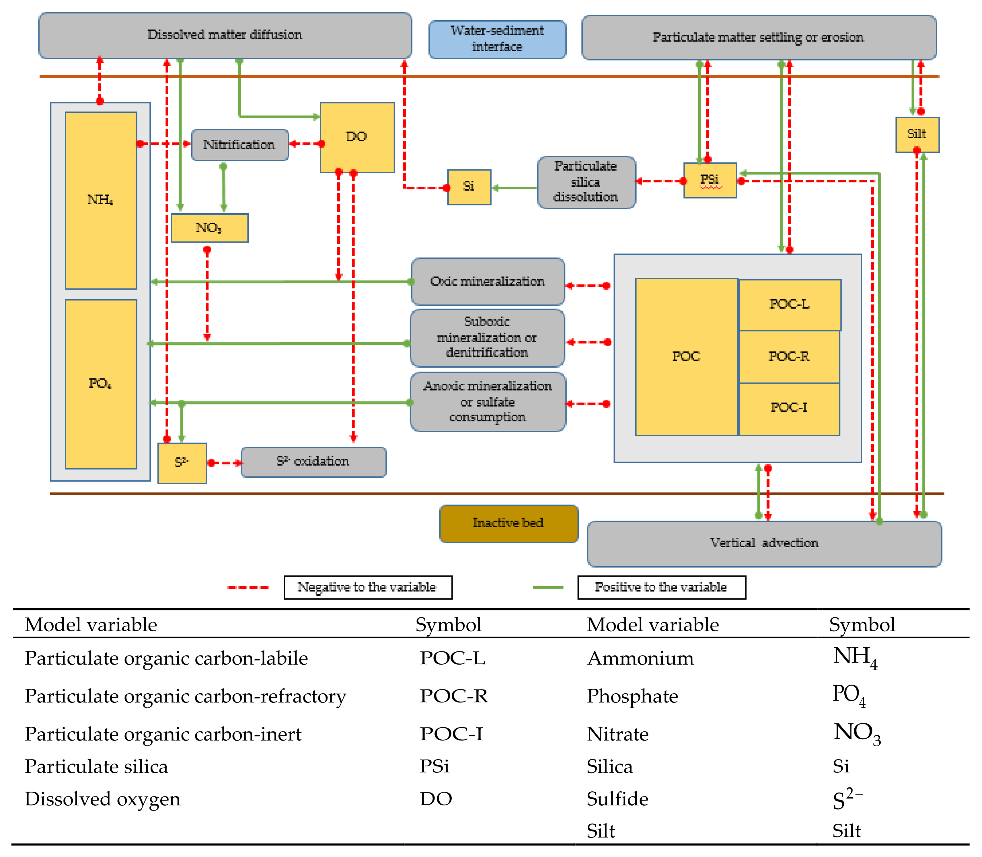
As with the pelagic model, the biochemical processes, their interconnections with other variables, and the benthic–pelagic coupling are shown in Figure 4. The main processes include mineralization under oxic, sub-oxic (denitrification), and anoxic (sulfate consumption) conditions, nitrification, oxidization of sulfide, and particulate silica dissolution. All the stoichiometric relationships associated with the biochemical processes are presented in Table 1. The expressions for the biochemical kinetic processes basically followed the formulae adopted in conventional models [19,20] (

Table A4. Kinetic equations for source terms in benthic model (see Appendix A (Table A1) for symbols).

Biochemical Process	Formulation
Particulate organic carbon	$\frac{d{B}_{\mathrm{POC}}}{dt}=\left[-\mathrm{Oxic}\_\mathrm{dec}-\mathrm{Anoxic}\_\mathrm{dec}\_{\mathrm{NO}}_3-\mathrm{Anoxic}\_\mathrm{dec}\_{\mathrm{SO}}_4\right]$
	$\frac{d{B}_{\mathrm{POC}}}{dt}=\left[-R_{B_{\mathrm{POC}}\_\mathrm{O}}-R_{B_{\mathrm{POC}}{\_\mathrm{NO}}_3}-R_{B_{\mathrm{POC}}{\_\mathrm{SO}}_4}\right]$
Aerobic carbon diagenesis:	$R_{B_{\mathrm{POC}}\_\mathrm{O}}=k_{B_{\mathrm{POC}}\_\mathrm{O}}{\theta }_{B_{\mathrm{POC}}}^{(T-20)}\left[\frac{B_{\mathrm{DO}}}{{\mathrm{K}}_{\mathrm{DO},B_{\mathrm{POC}}}+B_{\mathrm{DO}}}\right]B_{\mathrm{POC}}$
Anaerobic carbon diagenesis with nitrate as electron accepter or denitrification:	$R_{B_{{\mathrm{POC}\_\mathrm{NO}}_3}}=R_{B_{{\mathrm{NO}}_3}\_\mathrm{D}}{r}_{\mathrm{CN}\_\mathrm{D}}$ $R_{B_{{\mathrm{NO}}_3}\_\mathrm{D}}=k_{B_{{\mathrm{NO}}_3}\_\mathrm{D}}{\theta }_{B_{{\mathrm{NO}}_3}}^{(T-20)}\mathrm{MIN}\left[\frac{K_{\mathrm{DO},B_{\mathrm{POC}}}}{K_{\mathrm{DO},B_{\mathrm{POC}}}+B_{\mathrm{DO}}},\frac{B_{\mathrm{POC}}}{K_{\mathrm{dec},B_{\mathrm{POC}}}+B_{\mathrm{POC}}}\right]B_{{\mathrm{NO}}_3}$
Anaerobic carbon diagenesis with sulfate as electron accepter or sulfide production:	$R_{B_{{\mathrm{POC}\_\mathrm{SO}}_4}}=k_{B_{{\mathrm{POC}\_\mathrm{SO}}_4}}{\theta }_{B_{{\mathrm{POC}\_\mathrm{SO}}_4}}^{(T-20)}\mathrm{MIN}\left[\frac{K_{\mathrm{DO},B_{\mathrm{POC}}}}{K_{\mathrm{DO},B_{\mathrm{POC}}}+B_{\mathrm{DO}}},\frac{K_{B_{{\mathrm{NO}}_3},\mathrm{D}}}{K_{B_{{\mathrm{NO}}_3},\mathrm{D}}+B_{{\mathrm{NO}}_3}}\right]B_{\mathrm{POC}}$
Phosphorous	$\frac{d{B}_{{\mathrm{PO}}_4}}{dt}=\left[\left(\mathrm{Oxic}\_\mathrm{dec}+\mathrm{Anoxic}\_\mathrm{dec}\_{\mathrm{NO}}_3+\mathrm{Anoxic}\_\mathrm{deco}\_{\mathrm{SO}}_4\right)\mathrm{P}2\mathrm{C}\_\mathrm{ratio}\right]$
	$\frac{d{B}_{{\mathrm{PO}}_4}}{dt}=\left[\left(R_{B_{\mathrm{POC}}\_\mathrm{O}}+R_{B_{\mathrm{POC}}{\_\mathrm{NO}}_3}+R_{B_{\mathrm{POC}}{\_\mathrm{SO}}_4}\right)r_{\mathrm{PC}\_\mathrm{dec}}\right]$
Ammonia	$\frac{d{B}_{{\mathrm{NH}}_4}}{dt}=\left[\begin{array}{l}\left(\mathrm{Oxic}\_\mathrm{dec}+\mathrm{Anoxic}\_\mathrm{dec}\_{\mathrm{NO}}_3+\mathrm{Anoxic}\_\mathrm{dec}\_{\mathrm{SO}}_4\right)\mathrm{N}2\mathrm{C}\_\mathrm{ratio}\\ -\mathrm{Nitrification}\end{array}\right]$
	$\frac{d{B}_{{\mathrm{NH}}_4}}{dt}=\left[\left(R_{B_{\mathrm{POC}}\_\mathrm{O}}+R_{B_{\mathrm{POC}}{\_\mathrm{NO}}_3}+R_{B_{\mathrm{POC}}{\_\mathrm{SO}}_4}\right)r_{\mathrm{NC}\_\mathrm{dec}}-R_{B_{{\mathrm{NH}}_4}}\_\mathrm{N}\right]$
Nitrification:	$R_{B_{{\mathrm{NH}}_4}\_\mathrm{N}}=k_{B_{{\mathrm{NH}}_4}\_\mathrm{N}}{\theta }_{B_{{\mathrm{NH}}_4}\_\mathrm{N}}^{(T-20)}\left[\frac{B_{\mathrm{DO}}}{K_{\mathrm{DO},B_{{\mathrm{NH}}_4}}+B_{\mathrm{DO}}}\right]B_{{\mathrm{NH}}_4}$
Nitrate	$\frac{d{B}_{{\mathrm{NO}}_3}}{dt}=\left[\mathrm{Nitrification}-\mathrm{Denitrification}\right]$
	$\frac{d{B}_{{\mathrm{NO}}_3}}{dt}=\left[R_{B_{{\mathrm{NH}}_4}\_\mathrm{N}}-R_{B_{{\mathrm{NO}}_3}\_\mathrm{D}}\right]$
Particulate silica	$\frac{d{B}_{\mathrm{PSi}}}{dt}=\left[-\mathrm{Silica}\_\mathrm{production}\cdot \mathrm{Si}2\mathrm{PSi}\_\mathrm{ratio}\right]$
	$\frac{d{B}_{\mathrm{PSi}}}{dt}=\left[-R_{{\mathrm{B}}_{Si}\_\mathrm{Pro}}{r}_{\mathrm{Si}\_\mathrm{PSi}}\right]$
Dissolved silica production or particulate silica dissolution:	$R_{B_{\mathrm{Si}}\_\mathrm{Pro}}=k_{B_{\mathrm{Si}}}{\theta }_{B_{\mathrm{Si}}}^{(T-20)}\left[\frac{B_{\mathrm{PSi}}}{K_{B_{\mathrm{PSi}}}+B_{\mathrm{PSi}}}\right]\left[B_{\mathrm{Si},\mathrm{sat}}-B_{\mathrm{Si}}\right]$
Dissolved silica	$\frac{d{B}_{\mathrm{Si}}}{dt}=\left[\mathrm{Silica}\_\mathrm{production}\right]$
	$\frac{d{B}_{\mathrm{Si}}}{dt}=\left[R_{B_{\mathrm{Si}}}\_\mathrm{Pro}\right]$
Sulfide	$\frac{d{B}_{S^{2-}}}{dt}=\left[{\mathrm{Anoxic}\_\mathrm{dec}\_\mathrm{SO}}_4\cdot \mathrm{C}2\mathrm{S}\_\mathrm{ratio}-\mathrm{Sulfide}\_\mathrm{oxidation}\right]$
	$\frac{d{B}_{{\mathrm{S}}^{2-}}}{dt}=\left[R_{B_{\mathrm{POC}}{\_\mathrm{SO}}_4}{r}_{\mathrm{CS}\_\mathrm{dec}}-R_{B_{{\mathrm{S}}^{2-}}\_\mathrm{O}}\right]$
Sulfide oxidation:	$R_{B_{{\mathrm{S}}^{2-}}}\_\mathrm{oxi}=k_{B_{{\mathrm{S}}^{2-}}}\_\mathrm{oxi}{\theta }_{B_{{\mathrm{S}}^{2-}}}^{(T-20)}\left[\frac{B_{\mathrm{DO}}}{K_{{B_{\mathrm{S}}}^{2-},\mathrm{DO}}+B_{\mathrm{DO}}}\right]\frac{1}{r_{\mathrm{OS}\_\mathrm{oxi}}}$
Dissolved oxygen	$\frac{d{B}_{\mathrm{DO}}}{dt}=\left[\begin{array}{l}-\mathrm{oxic}\_\mathrm{dec}\cdot \mathrm{O}2\mathrm{C}\_\mathrm{ratio}-\mathrm{Nitrification}\cdot \mathrm{ON}\_\mathrm{ratio}\\ -\mathrm{Sulfide}\_\mathrm{oxidation}\cdot \mathrm{OS}\_\mathrm{ratio}\end{array}\right]$
	$\frac{d{B}_{\mathrm{DO}}}{dt}=\left[-R_{B_{\mathrm{POC}}\_\mathrm{O}}{r}_{\mathrm{OC}\_\mathrm{dec}}-R_{B_{{\mathrm{NH}}_4}\_\mathrm{nit}}{r}_{\mathrm{ON}\_\mathrm{nit}}-R_{{\mathrm{B}}_{{\mathrm{H}}_2\mathrm{S}}\_\mathrm{O}}{r}_{\mathrm{OS}\_\mathrm{oxi}}\right]$

).

2.8. Benthic Model Boundary Conditions and Numerical Procedure

Boundary conditions of the benthic model were considered at the bottom of the vertical active sediment column. Only the advection flux was applied for both dissolved and particulate matters at the bottom of the active sediment boundary, while the diffusion flux has been assumed as zero. The advection flux from bed to active sediment layer for dissolved matters was computed as

$${\mathrm{F}}_{i,j}^n={\left|{\omega }_{i,j}^n{B}_{i,j,k-1/2}^{n+1}{\varphi }_{i,j,k-1/2}^n\right|}_{k=(-\mathrm{kbe})}$$

(19)

where, $(i,j,k)$ represents the center of the grid point, $n$ is the time step, and $(\mathrm{kbe})$ is the number of layers in the sediment. Applying the upwind scheme

$${\omega }_{i,j}^n{B}_{i,j,k-1/2}^{n+1}=B_{i,j,k-1}^{n+1}〚{\omega }_{i,j}^n,0〛-B_{i,j,k}^{n+1}〚-{\omega }_{i,j}^n,0〛$$

(20)

defining an operator $〚A,B〛$ which denotes the greater of $A$ and $B$: when $A>B$ operator selects $A$ and vice versa [45]. Then,

$${\mathrm{F}}_{i,j}^n=|\left(B_{i,j,k-1}^{n+1}〚{\omega }_{i,j}^n,0〛-B_{i,j,k}^{n+1}〚-{\omega }_{i,j}^n,0〛\right){\varphi }_{i,j,k-1/2}^n{|}_{k=(-\mathrm{kbe})}$$

(21)

Assuming ${\left|B_{i,j,k-1}^{n+1}\right|}_{k=(-\mathrm{kbe})}={\left|B_{i,j,k}^{n+1}\right|}_{k=(-\mathrm{kbe})}$

$${\mathrm{F}}_{i,j}^n=|\left(〚{\omega }_{i,j}^n,0〛-〚-{\omega }_{i,j}^n,0〛\right)B_{i,j,k}^{n+1}{\varphi }_{i,j,k-1/2}^n{|}_{k=(-\mathrm{kbe})}$$

(22)

Evaluating the control volume face porosities explicitly and as the minimum between adjacent layer porosities, ${\varphi }_{i,j,k-1/2}^n=\mathrm{MIN}\left({\varphi }_{i,j,k}^n,{\varphi }_{i,j,k-1}^n\right)$.

$${\mathrm{F}}_{i,j}^n=|\left(〚{\omega }_{i,j}^n,0〛-〚-{\omega }_{i,j}^n,0〛\right)B_{i,j,k}^{n+1}\mathrm{MIN}\left({\varphi }_{i,j,k}^n,{\varphi }_{i,j,k-1}^n\right){|}_{k=(-\mathrm{kbe})}$$

(23)

Assuming ${\left|{\varphi }_{n,k-1}^m\right|}_{k=(-\mathrm{kbe})}={\left|{\varphi }_{n,k}^m\right|}_{k=(-\mathrm{kbe})}$

$${\mathrm{F}}_{i,j}^n=|\left(〚{\omega }_{i,j}^n,0〛-〚-{\omega }_{i,j}^n,0〛\right)B_{i,j,k}^{n+1}{\varphi }_{i,j,k}^n{|}_{k=(-\mathrm{kbe})}$$

(24)

Similarly, the advection flux from bed to sediment for particulate matters was computed as

$${\mathrm{F}}_{i,j}^n=|\left(〚{\omega }_{i,j}^n,0〛-〚-{\omega }_{i,j}^n,0〛\right)B_{i,j,k}^{n+1}\left(1-{\varphi }_{i,j,k}^n\right){|}_{k=(-\mathrm{kbe})}$$

(25)

For convenience, as in the pelagic model, the governing equations for dissolved and particulate scalar parameters were decomposed using a split operator as advection and diffusion and source terms. During discretization of the advection and diffusion equation, the vertical advection and vertical diffusion terms were discretized implicitly. The solution for the discretized equation was obtained by adopting the TDMA [45].

As in the solution method of source terms in the pelagic model, the finite difference method with the fourth order Runge–Kutta method, which gives approximate solutions of ordinary differential equations through an explicit approach, was used to obtain the solution for the source term equations in Table A4. Descriptions of the notations in the benthic model equations are listed in Table A1 and the model parameters for Tokyo Bay are listed in Table A2.

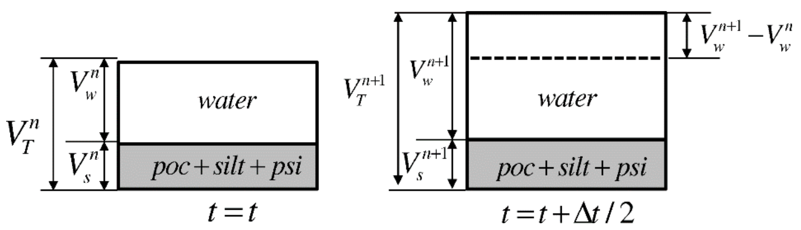
Bed formation was considered in order to compute the new layer thickness at every time step. The model was initialized with inorganic sediment, which is free from POC and becomes polluted with the POC accumulation from the water column. The accumulated POC changes the sediment porosity [39] and thereby the active sediment layer thickness with respect to the POCC.

It has been assumed that porosity, ${\varphi }^n$, increases to ${\varphi }^{n+1}$ ($>{\varphi }^n$) after time $\Delta t/2$ ($\Delta t$ is the time interval) with the increase in POCC in the sediment. This increases the total volume of the control volume from $V_t^n$ to $V_t^{n+1}$, as shown in Figure 5.

At $t=t$, the volume of dry sediment can be written as $V_s^n=\left(1-{\varphi }^n\right)V_T^n$.

At $t=t+\Delta t/2$, the volume of dry sediment can be written as $V_s^{n+1}=\left(1-{\varphi }^{n+1}\right)V_T^{n+1}$.

During the time $\Delta t/2$, it has been assumed that the change in the volume of dry sediment is negligible, and hence,

$$V_s^n=V_s^{n+1}$$

(26)

$$V_T^{n+1}=\mathrm{MF}\cdot V_T^n$$

(27)

$$\mathrm{MF}=\frac{(1-{\varphi }^n)}{(1-{\varphi }^{n+1})}$$

(28)

Then, the new layer thickness can be computed with a magnification factor $(\mathrm{MF})$ as

$$\Delta z^{n+1}=\mathrm{MF}\times \Delta z^n$$

(29)

Hence, with the change in POCC, the new porosity in the sediment was computed and the thickness of each sediment layer was renewed. As a result, the nutrient concentrations in each sediment layer were renewed for the new grid system at each time step.

2.9. Benthic and Pelagic Model Coupling

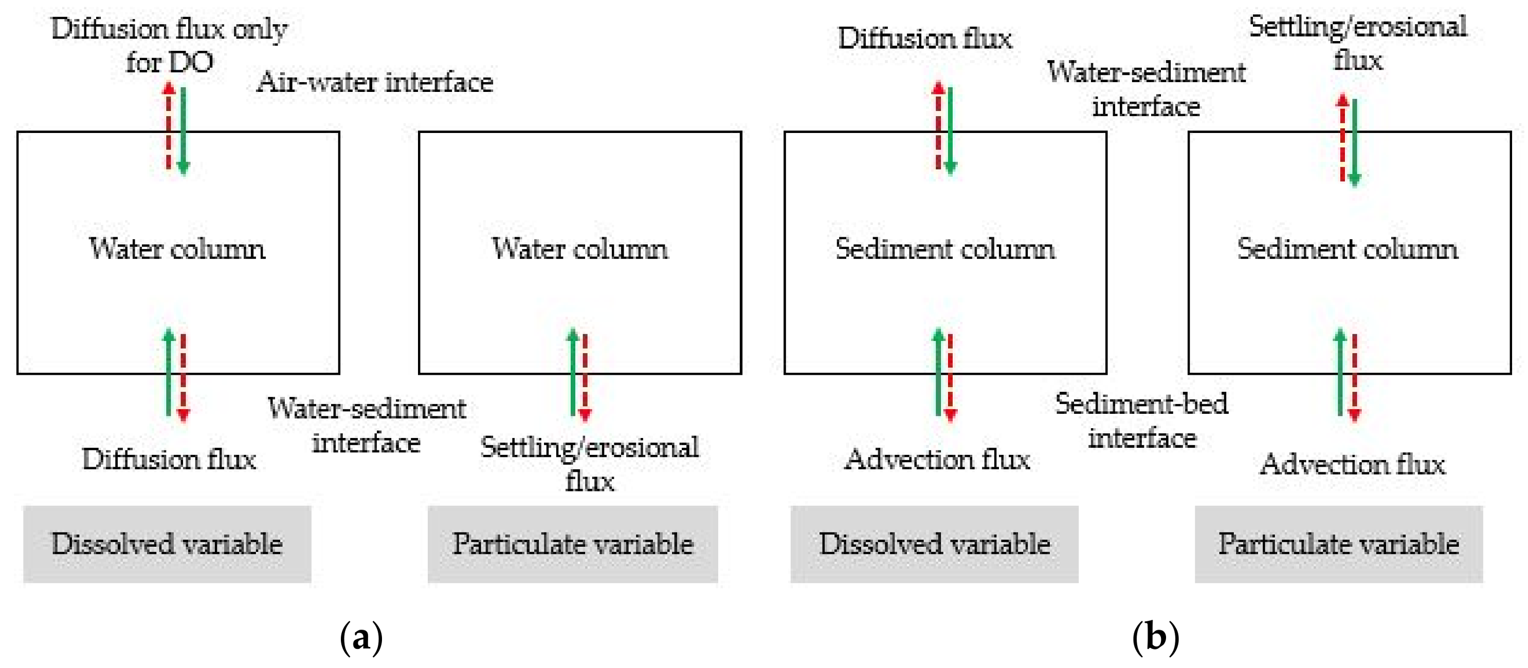
Model fluxes were computed at the air-water open boundary, bottom of the active sediment layer, and sediment–water interface (Figure 6). The benthic–pelagic model was coupled through the interaction layer flux at the sediment–water interface. The sediment–water interface has a diffusion flux of dissolved matter and a setting or erosional flux of particulate matter.

2.9.1. Diffusion Flux at Sediment–Water Interface

At the bottom of a water body or the sediment–water interface, dissolved nutrients and DO are constantly exchanged between the sediment bed and the overlying water through a process of diffusion, which is largely controlled by the difference in respective concentrations. However, the diffusion flux from sediment to water is controlled not only by the difference in concentration of nutrients but also by the oxygen concentration at the bottom of the water column. A zero diffusion flux for particulate matters at the sediment–water interface has been assumed. The transfer of diffusion flux from sediment to water occurs under anoxic condition, and the threshold value of the bottom layer oxygen has been considered as 2 g/m³ [53].

The diffusion flux of dissolved matter from sediment to water was computed as

$${\mathrm{F}}_{i,j}^n={\left|-K_{i,j,k+1/2}^n\frac{\partial B_{i,j,k+1/2}}{\partial z}{\varphi }_{i,j,k+1/2}^n\right|}_{k=0}$$

(30)

where $(i,j,k)$ represents the center of the grid point and $n$ is the time step.

Considering a diffusive boundary layer (DBL) with thickness $T_{DBL}$ (Figure 7), the diffusion flux can be computed as

$${\mathrm{F}}_{i,j}^n={\left|-K_{i,j,0+1/2}^n\frac{C_{i,j,DBL}^{n+1}-B_{i,j,0}^{n+1}}{\left(\Delta z_0^n/2+T_{DBL}\right)}{\varphi }_{i,j,0+1/2}^n\right|}_{k=0}$$

(31)

where $\Delta z_0$ is the thickness of the surface sediment layer and $T_{DBL}$ is the thickness of the DBL in the water column, which depends on the thickness of the bottom layer of the water column and has been considered as a tuning parameter of the model.

2.9.2. Particulate Matter Settling or Resuspension

Particulate matters settle down through the water column and depending on the BSS ${\tau }_{\mathrm{b}}$, critical BSS on deposition ${\tau }_{\mathrm{D}}$, and critical BSS on erosion ${\tau }_{\mathrm{E}}$, they accumulate on the sediment bed or erode from it. The settled POC undergoes diagenesis through decomposition, resulting in hypoxic or anoxic conditions in the water column. Aerobic or anaerobic decomposition of these accumulated POC results in the buildup of high concentrations of phosphate and ammonium in the sediment and, under anoxic conditions, those nutrients are released to the overlying water. Hence, accurate modeling of the particulate matter settling in the water column is an important component for both water quality and sediment quality analysis.

The settling term was discretized with an implicit upwind scheme and the depositional flux, $F_{\mathrm{D}}$ [40], was computed as

$$F_{\mathrm{D}}=\left\{\begin{array}{ll}{\dot{\sigma }}_{sij\left(1-1/2\right)}{C}_{ij\left(1-1/2\right)}^{n+1}\left(1-\frac{{\tau }_{\mathrm{b}}}{{\tau }_{\mathrm{D}}}\right)& {\tau }_{\mathrm{b}}<{\tau }_{\mathrm{D}}\\ 0& {\tau }_{\mathrm{b}}>{\tau }_{\mathrm{D}}\end{array}\right\}$$

(32)

while the erosional flux, $F_{\mathrm{E}}$ [5] was computed as

$$F_{\mathrm{E}}=\left\{\begin{array}{ll}{E}_0\left(\frac{{\tau }_{\mathrm{b}}}{{\tau }_{\mathrm{E}}}-1\right)& {\tau }_{\mathrm{b}}>{\tau }_{\mathrm{E}}\\ 0& {\tau }_{\mathrm{b}}<{\tau }_{\mathrm{E}}\end{array}\right\}$$

(33)

where $E_0$ is the empirical erosion rate parameter. Because the erosional flux was computed as the total eroded material from the sediment, it has been separated into the corresponding particulate matter according to their mass fraction, ${\mathrm{F}}_{\mathrm{M},B}$, which is computed as the ratio of mass of each particulate matter, ${\mathrm{M}}_B$ to the total mass eroded from the sediment, ${\mathrm{M}}_{\mathrm{T}}$.

$${\mathrm{F}}_{\mathrm{M},B}=\frac{{\mathrm{M}}_B}{{\mathrm{M}}_{\mathrm{T}}}$$

(34)

The eroded total mass can be replaced with the bulk density ${\rho }_{\mathrm{bulk}}$, and the total volume $V_{\mathrm{T}}$ of the eroded sediment. The mass fraction of any particulate matter in the sediment can be written as

$${\mathrm{F}}_{\mathrm{M},B}=\frac{{\mathrm{M}}_B}{{\rho }_{\mathrm{bulk}}{\mathrm{V}}_{\mathrm{T}}}$$

(35)

The concentration of the state variables has been defined as mass over unit control volume $B={\mathrm{M}}_B{/\mathrm{V}}_{\mathrm{T}}$. Then, the mass fraction of each particulate matter that erodes from the sediment can be represented as

$${\mathrm{F}}_{\mathrm{M},B}=\frac{B}{{\rho }_{\mathrm{bulk}}}$$

(36)

Assuming that erosion occurs only from the surface layer of the sediment,

$${\rho }_{\mathrm{bulk}}={\left|B_{\mathrm{Silt}}(i,j,k)+\left(B_{\mathrm{POC}}(i,j,k)+B_{\mathrm{PSi}}(i,j,k)\right)+\varphi (i,j,k){\rho }_{\mathrm{w}}\right|}_{k=0}$$

(37)

where ${\rho }_{\mathrm{w}}$ is the density of the sea water.

3. Model Application to Tokyo Bay

Tokyo Bay is one of the most polluted, semi-enclosed, shallow coastal embayments in the world. It is located in the central part of the main island of Japan, has a mean water depth of 15 m, and covers an area of 150 km². The upwelling of the anoxic bottom water, which creates blue tides resulting in substantial economic losses to coastal fisheries, is still unsolved. Given the availability of data, Tokyo Bay was selected for the calibration and validation of the model.

3.1. Model Grid System

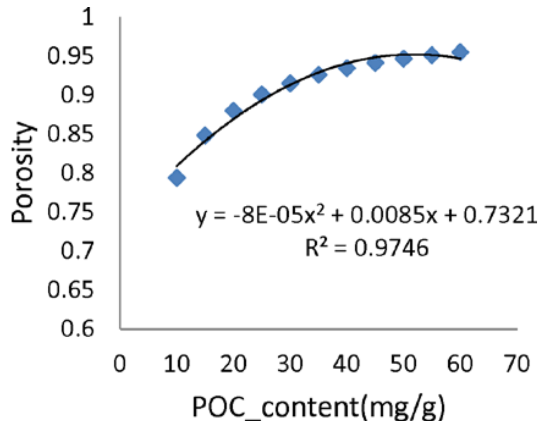
Model grids for both benthic and pelagic sub models were generated to coincide to each other with (2000 × 2000 m) horizontal resolution, while the vertical grids were generated independently. The pelagic model was composed of 20 $\sigma$-layers, and the benthic model was composed of 25 layers with different layer thicknesses in vertical direction. Based on the data analysis [39], the relationship between porosity and POCC was derived as shown in Figure 8, and it was applied to compute the new layer thickness in the benthic model at every time step with respect to POCC.

3.2. Initial Conditions

Because the time variable solutions for both the water and sediment state variables require initial conditions to start the computation, they were given as the concentrations at $t=0$. The pelagic model initial conditions for all the state variables were given uniformly based on the available data [43] (Table 2). The benthic model was initialized with zero initial values for all the state variables, including POC, which was considered as a completely inorganic sediment.

3.3. Boundary Conditions

Boundary conditions were considered at the bay mouth, river and sewage mouths, free water surface, and bottom of the sediment layer. The pelagic model boundary conditions for all the state variables at the bay mouth were given based on the available data [43] (Table 2).

The locations of the 12 river boundaries and 11 sewage outfall point sources at the mesh were considered as shown in Figure 9, and the corresponding discharges and nutrient concentrations have been obtained from the available government sources. Boundary conditions at the free water surface were set to zero, except for DO, while the boundary conditions at the bottom of the sediment for the dissolved and particulate state variables have been computed with the governing equations of vertical advection and diffusion. The model was forced by hourly meteorological data (Figure 10), which includes rainfall, air temperature, solar radiation, air pressure, vapor pressure, relative humidity, cloud cover, wind vector, and instantaneous tidal motion.

3.4. Model Calibration and Validation

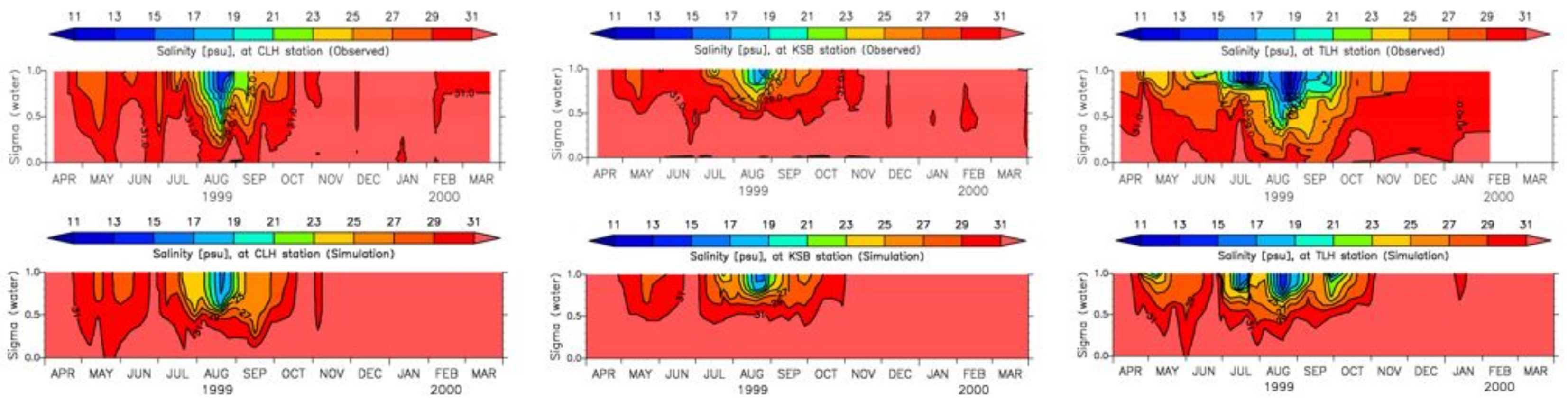
Computation started from 1 January and continued for a one-year period until 31 December. Each model was run for a one-year period and 200 models were run with changing initial conditions to obtain long-term results of 200 years. The output of the last time step of each year was used as the initial conditions of the next year model with the same boundary conditions. A 3D output was generated for all the state variables at every noon with a one-day interval. The output was generated at the three designated points where data were collected—namely, CLH, KSB, and TLH—as shown in Figure 1, at every one-hour interval and at the designated dates when data was collected. The model was validated for vertical distributions of water quality for the period from April 1999 to March 2000 [43] and regarding spatial distribution of POCC for the year 2001 [39].

4. Results

4.1. Water Quality

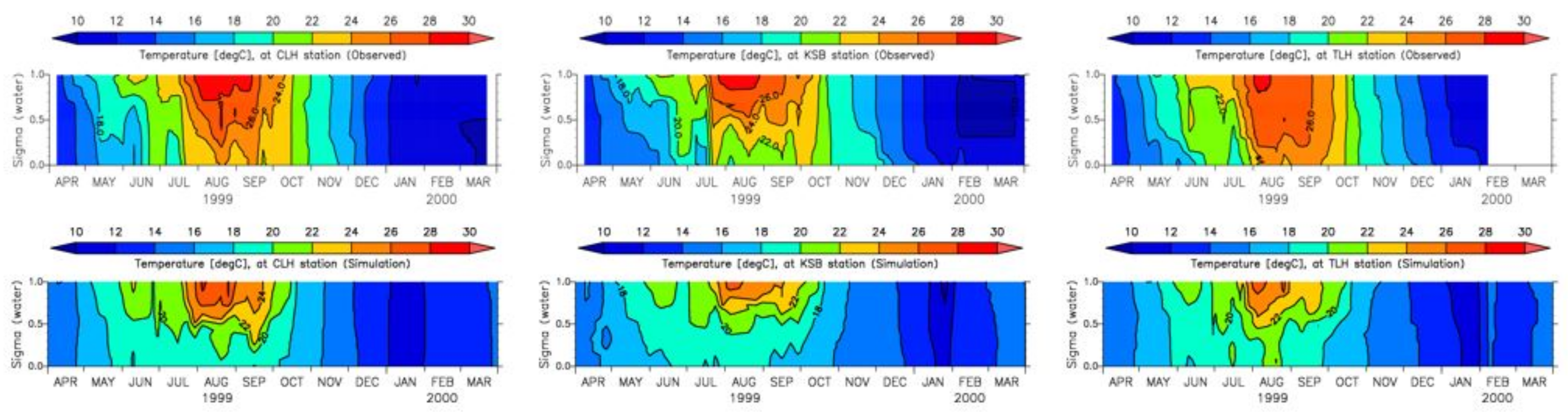
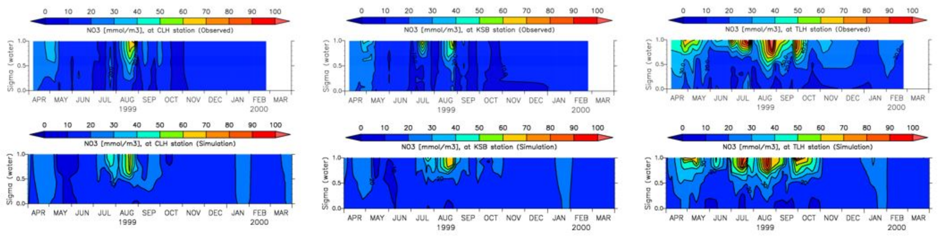
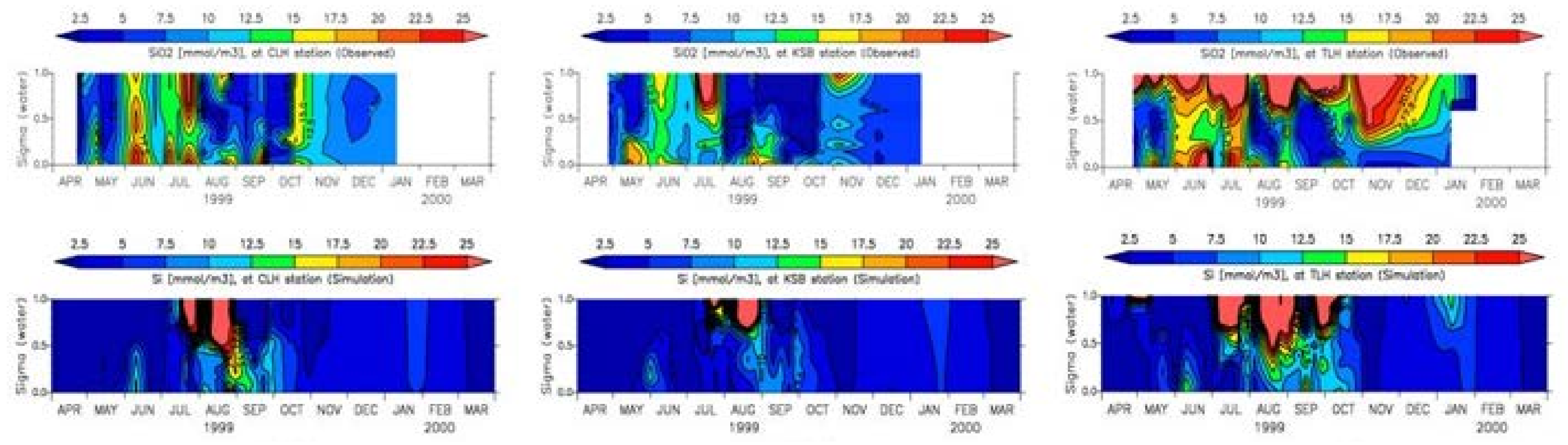
The model was validated for vertical distributions of the water quality parameters of salinity, temperature, chlorophyll a, DO ammonium, phosphate, nitrate, and silica, at the three locations of CLH, KSB, and TLH, for the period from April 1999 to March 2000 [43].

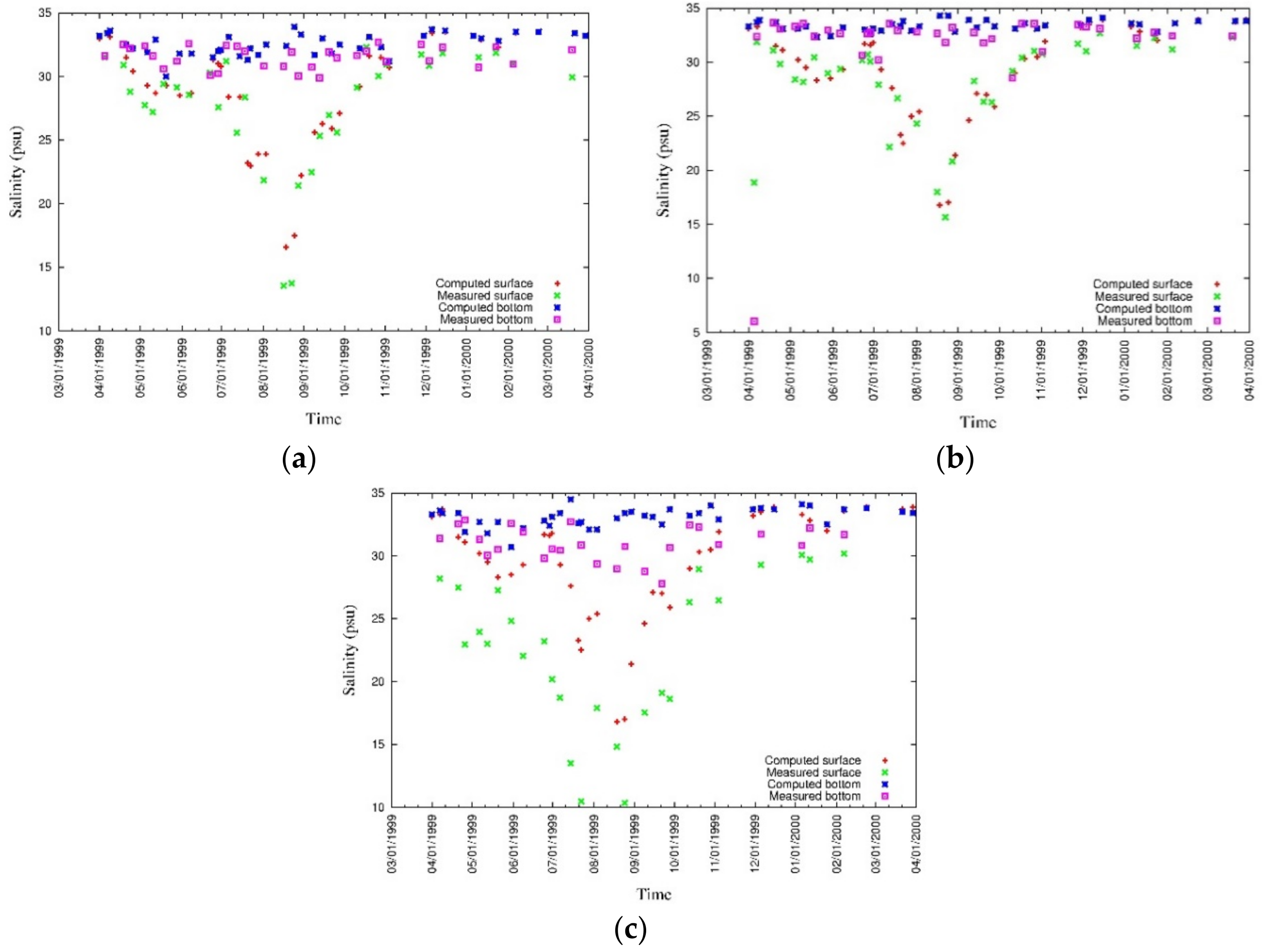
Salinity and temperature are two important parameters in water quality modeling. Water stratification, which affects water column mixing, is controlled by both salinity and temperature. The inflow of fresh water changes the salinity of the surface water, and it tends to move the surface water out from the bay mouth, resulting in highly saline water intrusion to the bottom of the water column moving the bottom anoxic water mass towards the head of the bay. Kinetic rates of nutrient transformation are influenced by temperature as all the kinetic equations in the model have positive correlation coefficients with temperature. Moreover, primary production is also controlled by the water temperature as growth rate is increased with the increase in temperature to an optimum level. The vertical distributions of modeled and measured salinity at three locations are shown in Figure 11 while surface and bottom values have been plotted in Figure 12 [43].

The highest discrepancies are shown at TLH location which is close to a river mouth. Surface salinity, especially near the river mouths, is highly influenced by river discharges, and thus, accurate river discharge data can further improve the reproducibility of salinity.

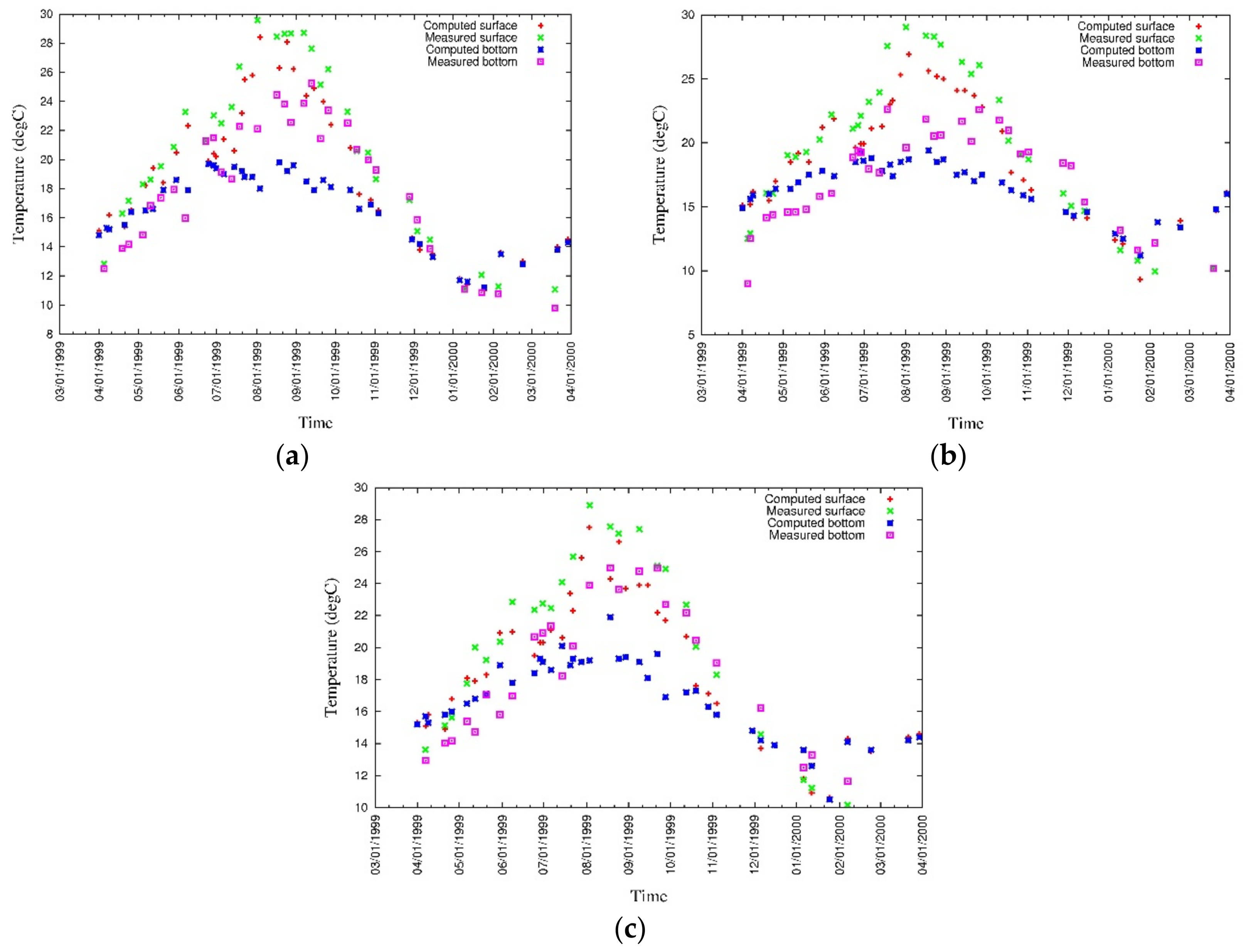
The vertical distributions of modeled and measured temperature at three locations are shown in Figure 13 while surface and bottom values have been plotted in Figure 14 [43]. According to the measured and simulated values of surface and bottom temperature at three locations, the values differ considerably during the summer. Surface heat transfer through the water column is significant to model accurate temperature distribution at the bottom layer.

Phytoplankton biomass and spatiotemporal distribution are mainly controlled by light, temperature, nutrient supply, and hydrodynamic characteristics [54,55,56,57]. Light is the most important limiting factor for photosynthesis. The effect of light on primary production was described by the most frequently used Steele formula [58] in the model. The effect of temperature on primary production was modeled as primary production increases until an optimum temperature is reached, and it is inhibited after further temperature increment [20]. Nitrogen, phosphate, and silica are the three essential nutrients for primary production, though silica is used only by diatoms. The limiting function of the nutrients was modeled according to Liebig’s law of the minimum [58].

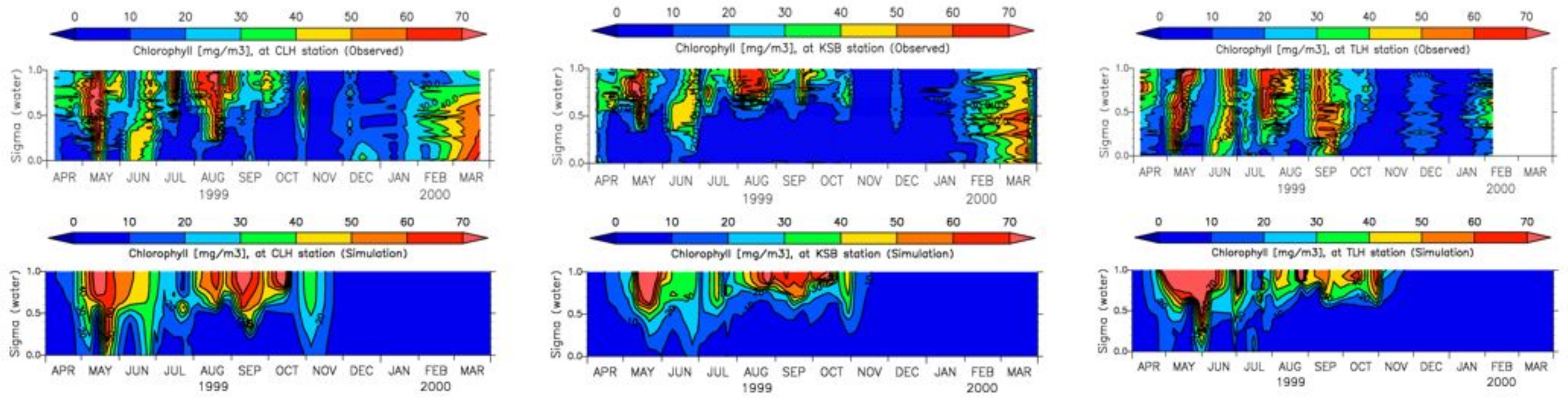
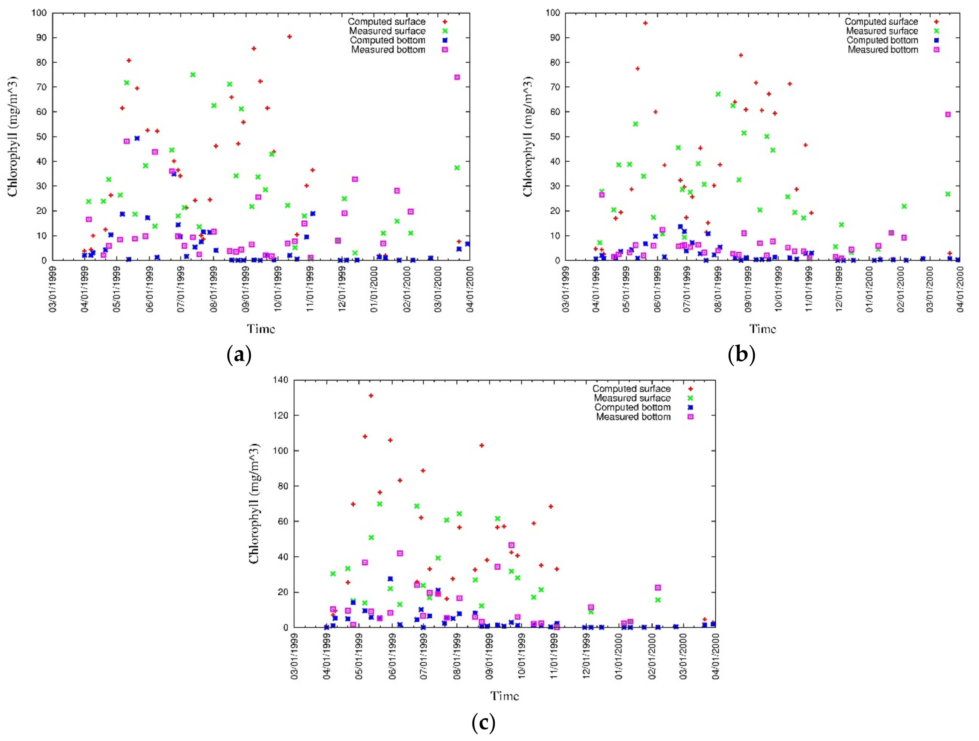
Three seasonal blooms, which appear every year in Tokyo Bay, have been modeled for the seasons of spring, summer, and winter (Figure 15). Though the spring bloom was underestimated at the beginning, the strongest spring bloom appeared in May throughout the water column owing to relatively calm water, which allows satisfactory penetration of light. The summer bloom was mainly concentrated in surface layers owing to the stratification and lower light penetration through the water column. During winter, the water column is well mixed and calm with sufficient light penetration capability. Even the winter bloom was modelled for lower limiting temperatures, it was considerably underestimated. Measured and simulated values of surface and bottom chlorophyll a at three locations are shown in Figure 16 [43]. Discrepancies are considerably high at the surface owing to environmental forcing such as solar radiation and mix layer thickness.

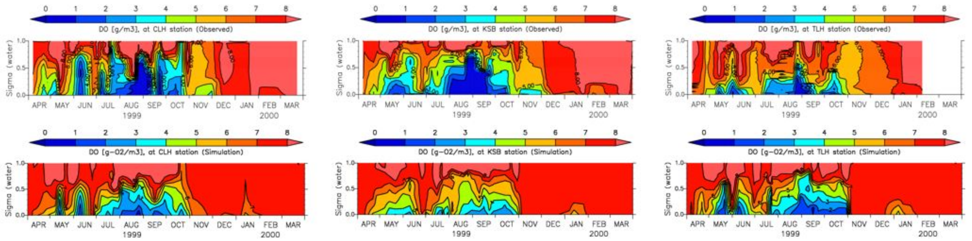
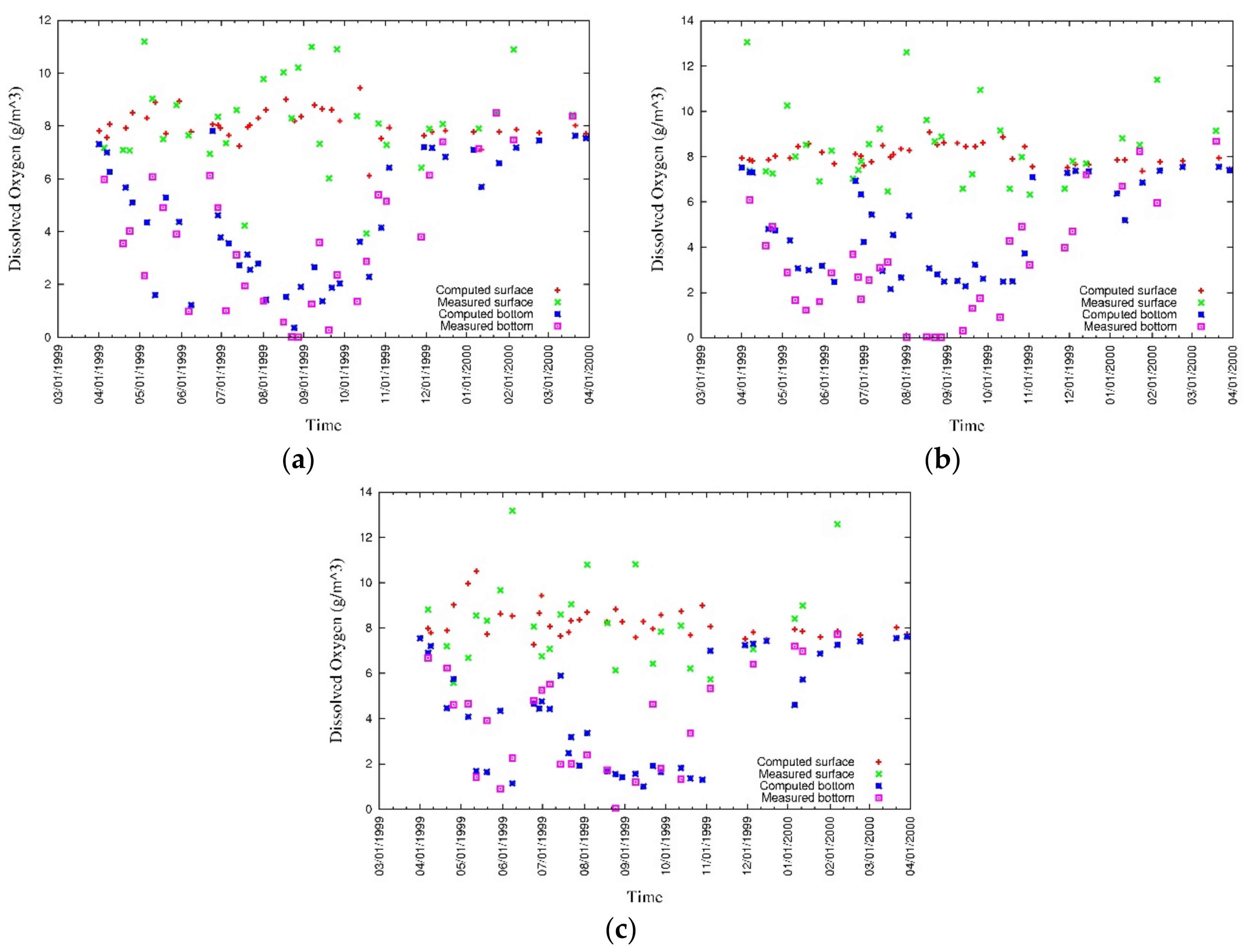
Severe hypoxia, which is typically defined as DO concentration below 2 g/m³ [53], especially appears during summer in Tokyo Bay. Seasonal hypoxia at the three locations in Tokyo Bay has been well reproduced qualitatively, though it was underestimated to some extent (Figure 17). Measured and simulated values of surface and bottom DO at three locations (Figure 18) show considerable discrepancies in both surface and bottom layers [43]. As the reproducibility of seasonal hypoxia in the water column has a strong correlation with the reproducibility of chlorophyll a, accurate modeling of chlorophyll a will improve the DO model. Moreover, it has been noticed that the surface DO concentration is highly affected by both primary production and the saturated concentration of DO.

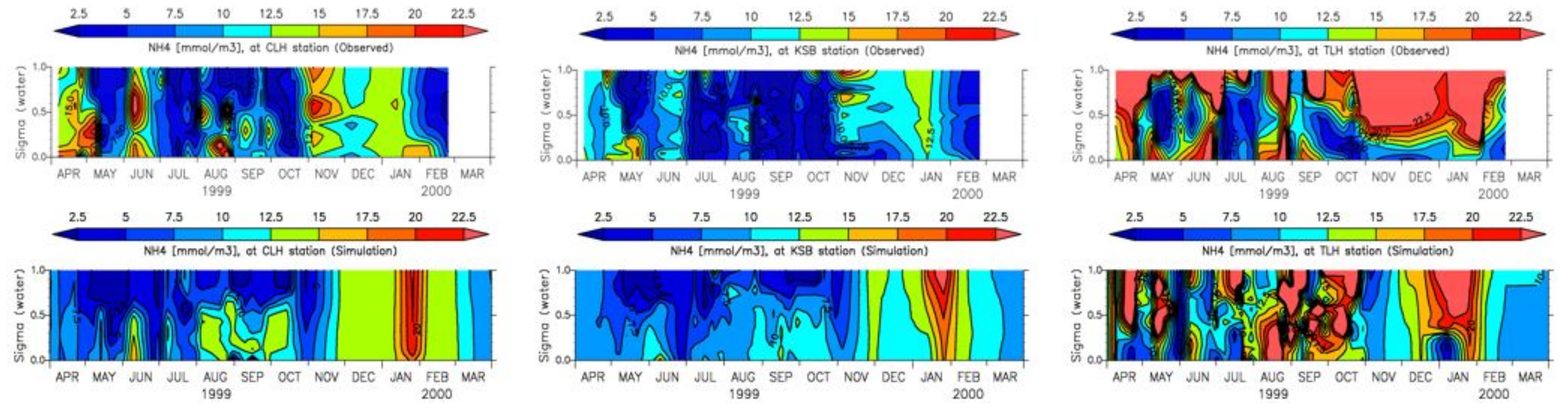
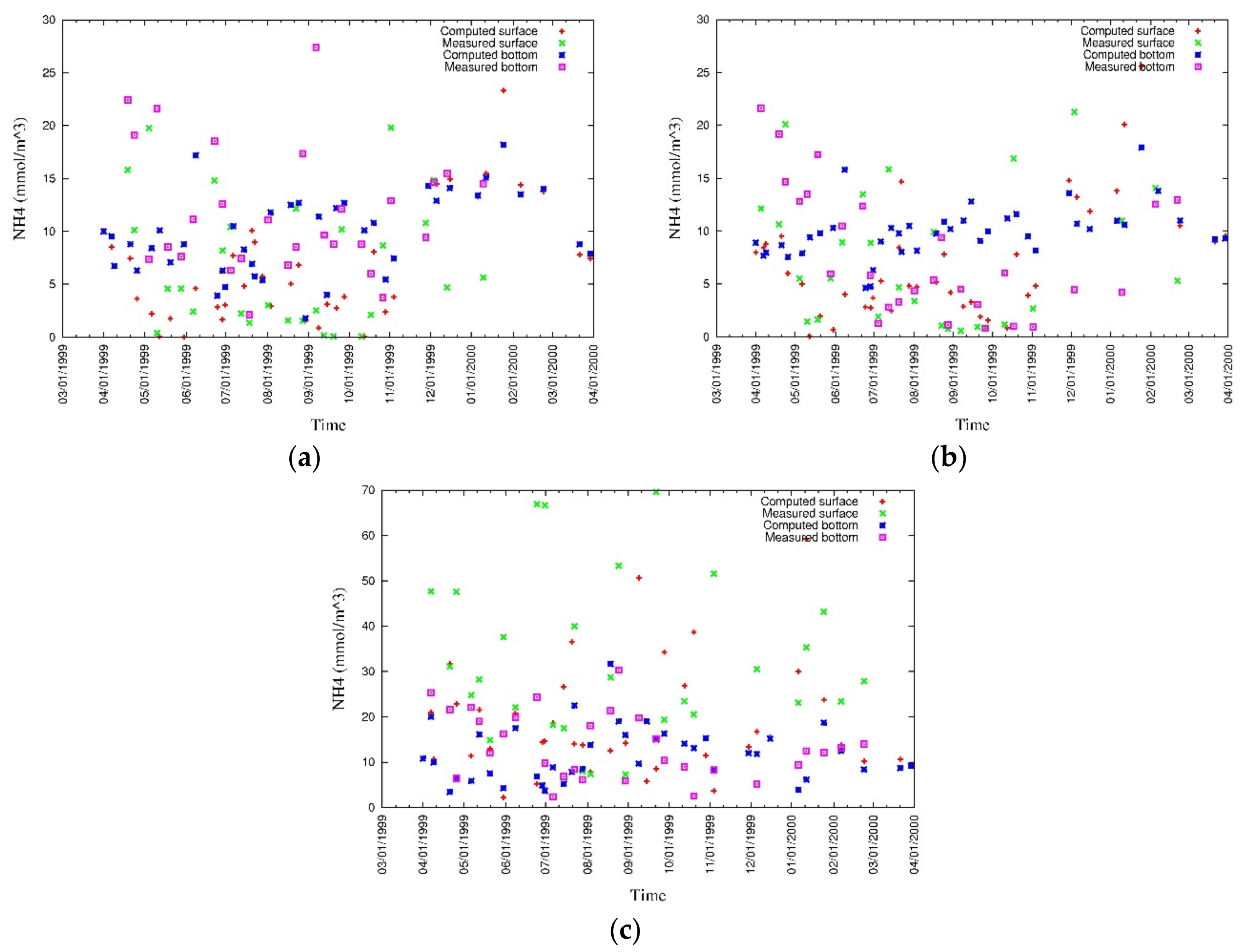
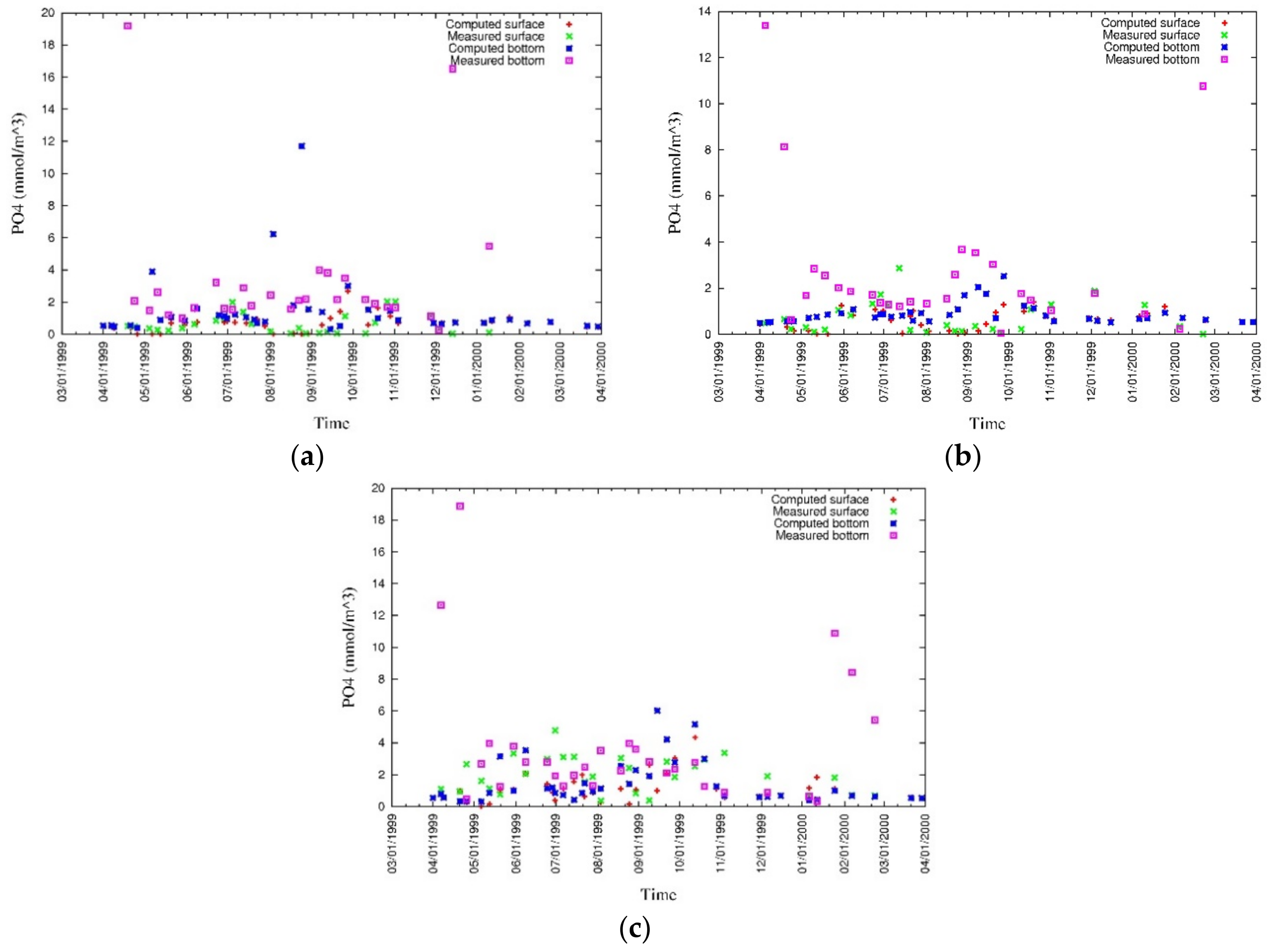
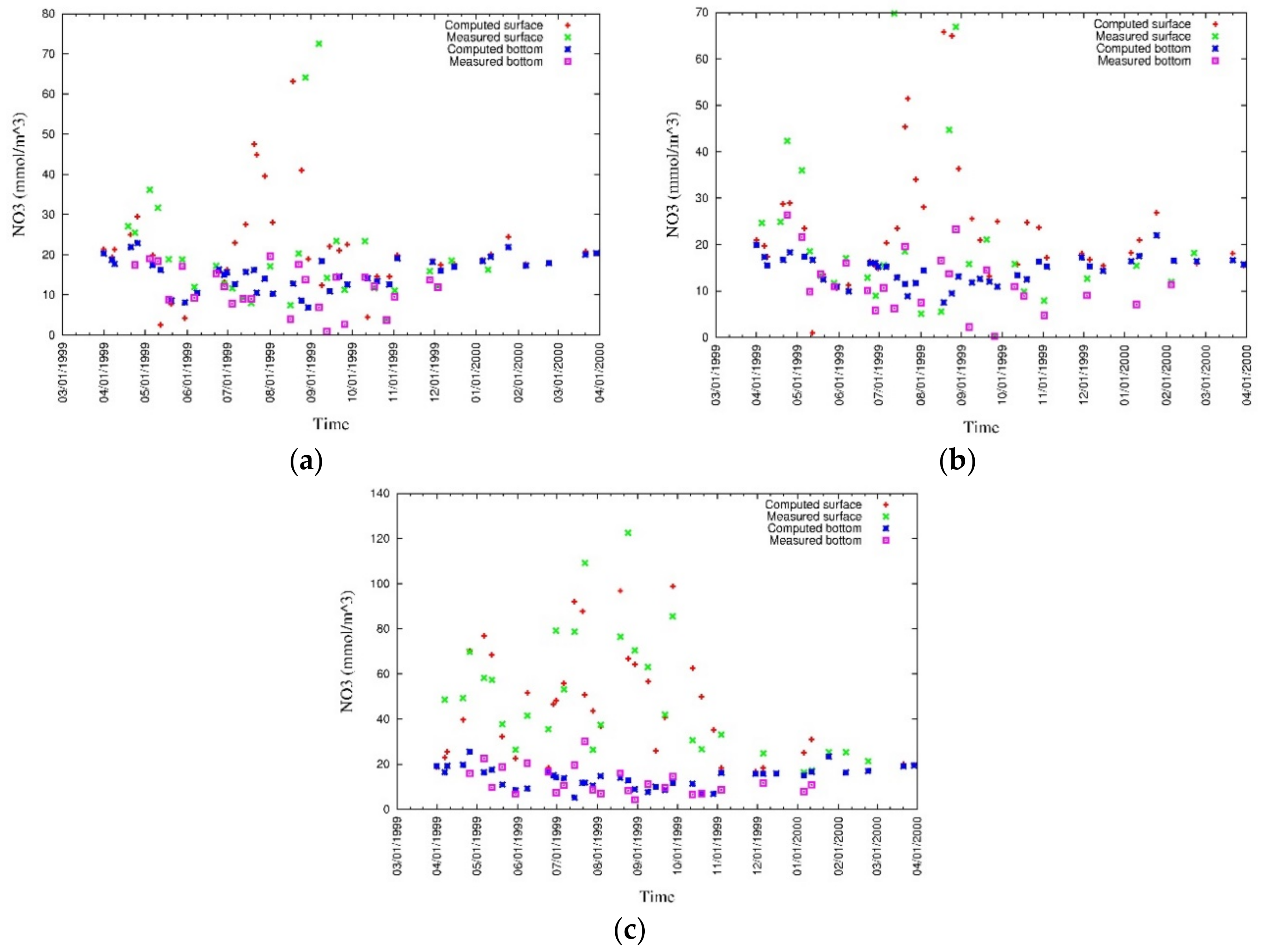
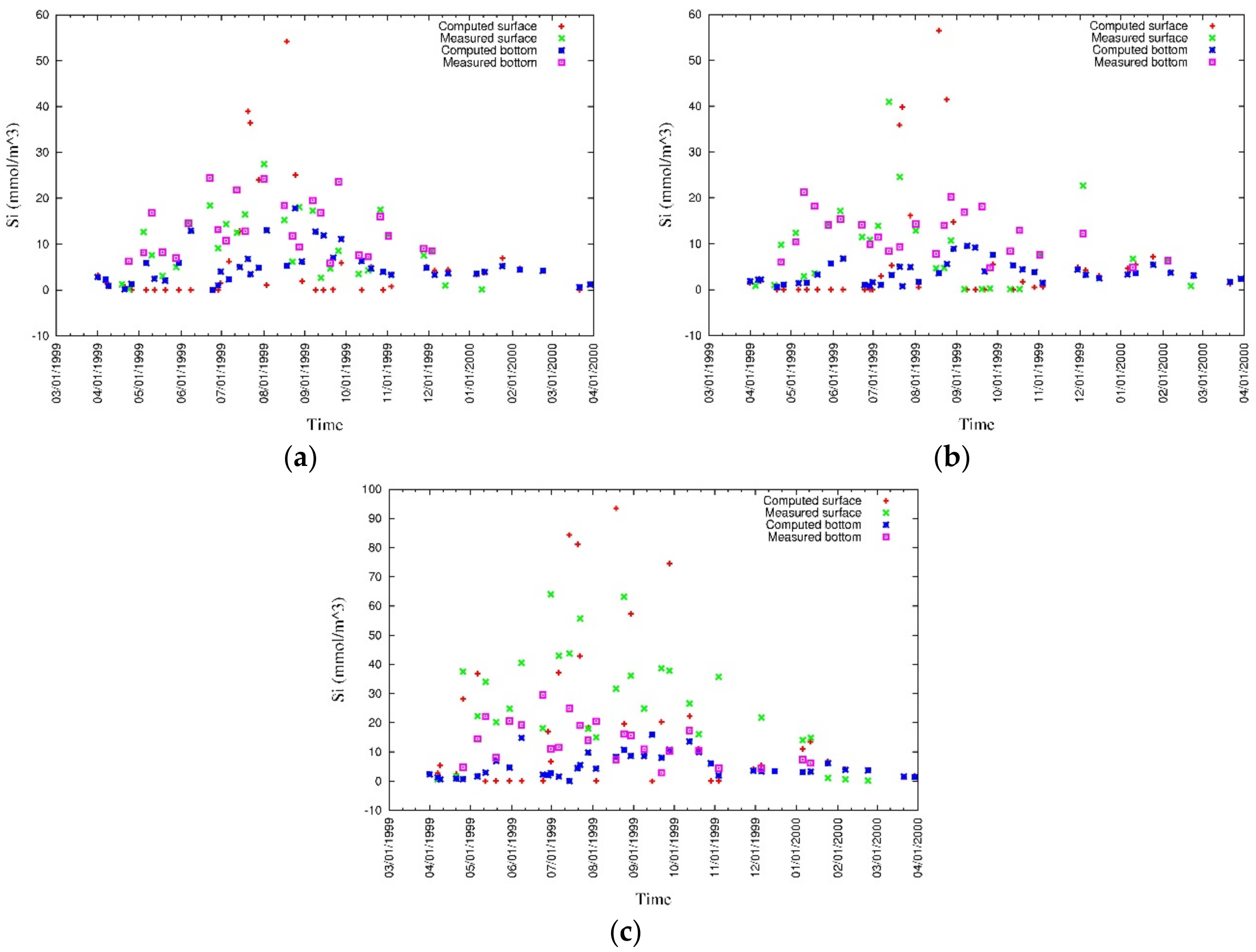
The vertical distributions, and surface and bottom values of modeled and measured ammonia (Figure 19 and Figure 20), phosphate (Figure 21 and Figure 22), nitrate (Figure 23 and Figure 24), and silica (Figure 25 and Figure 26) were analyzed during this study [43]. Discrepancies in surface nutrient concentrations suggest inaccuracies in river discharges and their concentrations, which require to be corrected in future studies. Moreover, surface nutrient concentrations are sensitive to the phytoplankton model. At the bottom, the nutrient flux is released under anoxic condition, and as the DO concentration at the bottom of the water column is overestimated in some degree, the release of nutrients from sediment to water is underestimated. Furthermore, it has been confirmed by sensitivity analysis that the release of phosphorus from the sediment is controlled by the attached and dissolved fractions of phosphors within it. The ammonia model is controlled by many factors and careful sensitivity analysis of parameters is further needed for the improvement of the model.

4.2. Sediment Quality

The sediment bed in Tokyo Bay has been formed over a long period. Some argue that water pollution in Tokyo Bay is the result of an excess of nutrients in the water column. However, government efforts to reduce nutrient inflows to the bay have not yet given the expected reduction levels of pollution in the bay water. Hence, it has been deeply discussed among stakeholders whether the polluted sediment bed has a significant effect on bay water quality. It is expected that water quality will be improved in the future through the improvement of sediment quality, and therefore, a detailed analysis of sediment quality in the bay is of high importance.

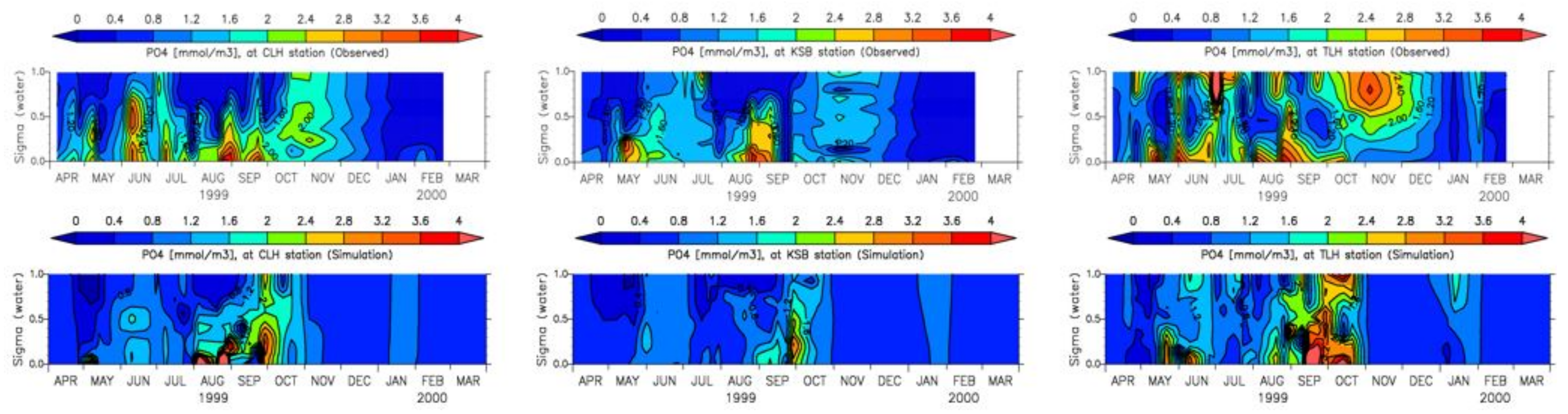
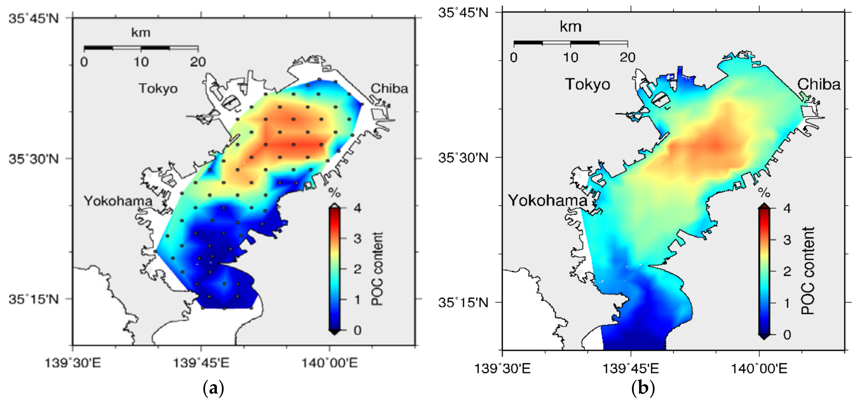
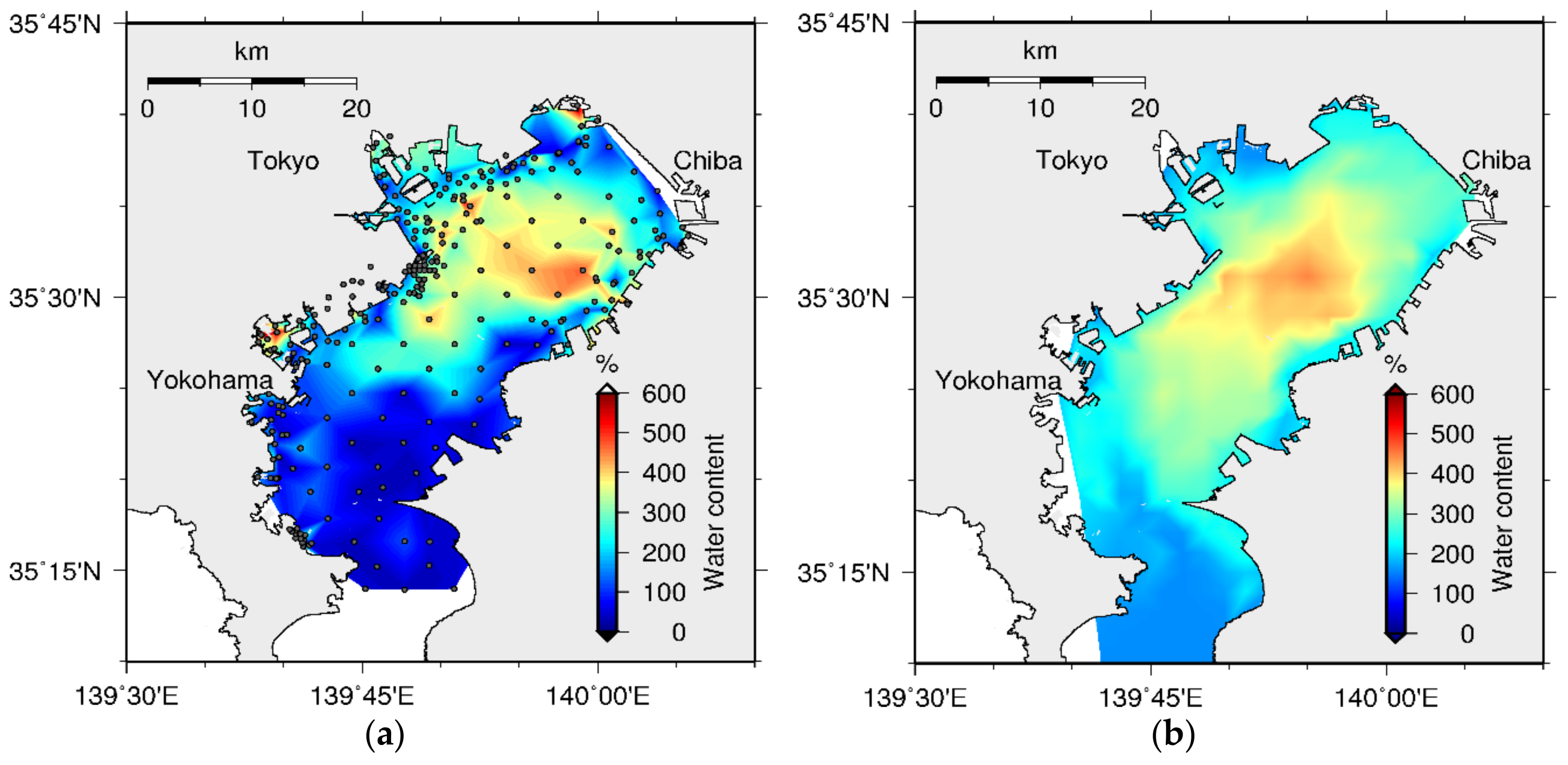
The available data has confirmed that the sediment water pollution is accumulated at the central part of the bay, and it has a positive correlation with the bottom water quality. The model was validated for the spatial distribution of POCC in the year 2001 [39]. The computed spatial distributions of POCC (Figure 27) and WC (Figure 28) were basically consistent with those in the measurements, which show high concentration towards the central part of the bay. Moreover, the positive correlation between POCC and WC, which has been revealed by the data [38], was confirmed through this modeling.

5. Discussion

5.1. Environmental Controls of Water Quality

The distribution of phytoplankton community and thereby water quality is governed by a number of physical, chemical, and biochemical processes such as advection, diffusion, stratification, vertical mixing, water temperature, light, nutrient supply, and establishment of weather fronts [59]. Moreover, all these processes are driven by meteorological forces such as air temperature, rainfall, and wind [60,61].

According to Figure 11 and Figure 13, the period from June to October can be characterized as the development of stratification of salinity and temperature, while the period from October to March can be characterized as uniform salinity and temperature owing to vertical mixing. These results represent the data well [43] with minor quantitative discrepancies, especially near the river mouths. The surface salinity near the river mouths is highly influenced by river discharges, and thus, accurate river discharge data can further improve the reproducibility of salinity. Moreover, as both salinity and temperature have been modeled under uniform spatial and vertical boundary conditions, the improvement in boundary conditions will further improve their reproducibility.

Figure 15 shows high phytoplankton bloom during late spring and summer, whereas declined phytoplankton bloom is observed during winter. A similar variation in phytoplankton bloom during late spring and summer was examined by Bouman et al. [62] for Tokyo Bay, and they confirmed that the heavy precipitation and high surface temperature during that season give rise to a highly stratified water column and consequently stimulated a series of phytoplankton blooms. Moreover, the short term dynamics of the phytoplankton community is closely coupled with the environmental forcing, and the degree of coupling is stronger when the solar radiation is greater [27]. Phytoplankton can increase rapidly even under average solar radiation if the optimum conditions of mixed-layer thickness and eutrophic zone are met [28]. Hence, this seasonal variation of phytoplankton reflects not only seasonal changes in temperature [63,64] but also seasonal variations in solar radiation. As a result, a weakly stratified and deeply mixed water column leads to a rapid decline in phytoplankton biomass under the light-limited growth conditions during the winter. During the period of November to March, where vertical mixing is high and nutrients are relatively abundant, chlorophyll a concentration is remarkably low. This suggests that the available nutrients were not utilized by the phytoplankton owing to some other physical condition. Physical conditions such as the north-wind induced outflow and vertical mixing have also been identified as causes for dilution of phytoplankton and termination of blooms in Tokyo Bay [28]. In order to overcome the discrepancies in the phytoplankton model, accurate modeling of light penetration and inclusion of accurate physical conditions, such as wind-induced outflow, have to be considered in futures studies.

Oxygen depleted water is formed at the bottom of the water column during the stratification period [27]. Oxygen-depleted bottom water, especially during summer, results from the increase in oxygen consumption by the benthic system and decrease in vertical mixing [6]. Figure 17 shows that from June to October, when the water column is stratified owing to salinity and temperature and the phytoplankton bloom is high, DO depletion occurs at the bottom of the water column, and this confirms the data [43]. The model results underestimate the hypoxia, especially during summer. This is expected to improve through the accurate modeling of phytoplankton as there is a direct correlation between phytoplankton blooms and DO depletion at the bottom of the water column.

Nutrient loads have been found to be high in the surface water owing to external nutrient supply through river and sewer water, and they are depleted by pulses of primary production [27,65]. Nutrient concentrations in the model (Figure 19, Figure 21, Figure 23 and Figure 24) are basically consistent with the data [43]; however, quantitative discrepancies appear both at the surface and at the bottom of the water column. The surface discrepancies are mainly due to inaccuracies in the river inflows and their concentrations. For instance, high surface nutrient concentrations can especially be seen at TLH, where the collected data location is near a river mouth. Improvement in the underestimation of hypoxia and inclusion of benthic animals to the sediment model in future studies are expected to improve the discrepancies in nutrient concentrations in the bottom water.

5.2. Bed Formation

Modeling of benthic–pelagic coupled water quality is often challenging considering the scarcity of available sediment data. To overcome this difficulty, we have proposed a novel approach to initialize the sediment model with totally inorganic sediment. Sediment becomes polluted and sediment nutrients are accumulated over time with the accumulation of POC from the overlying water column.

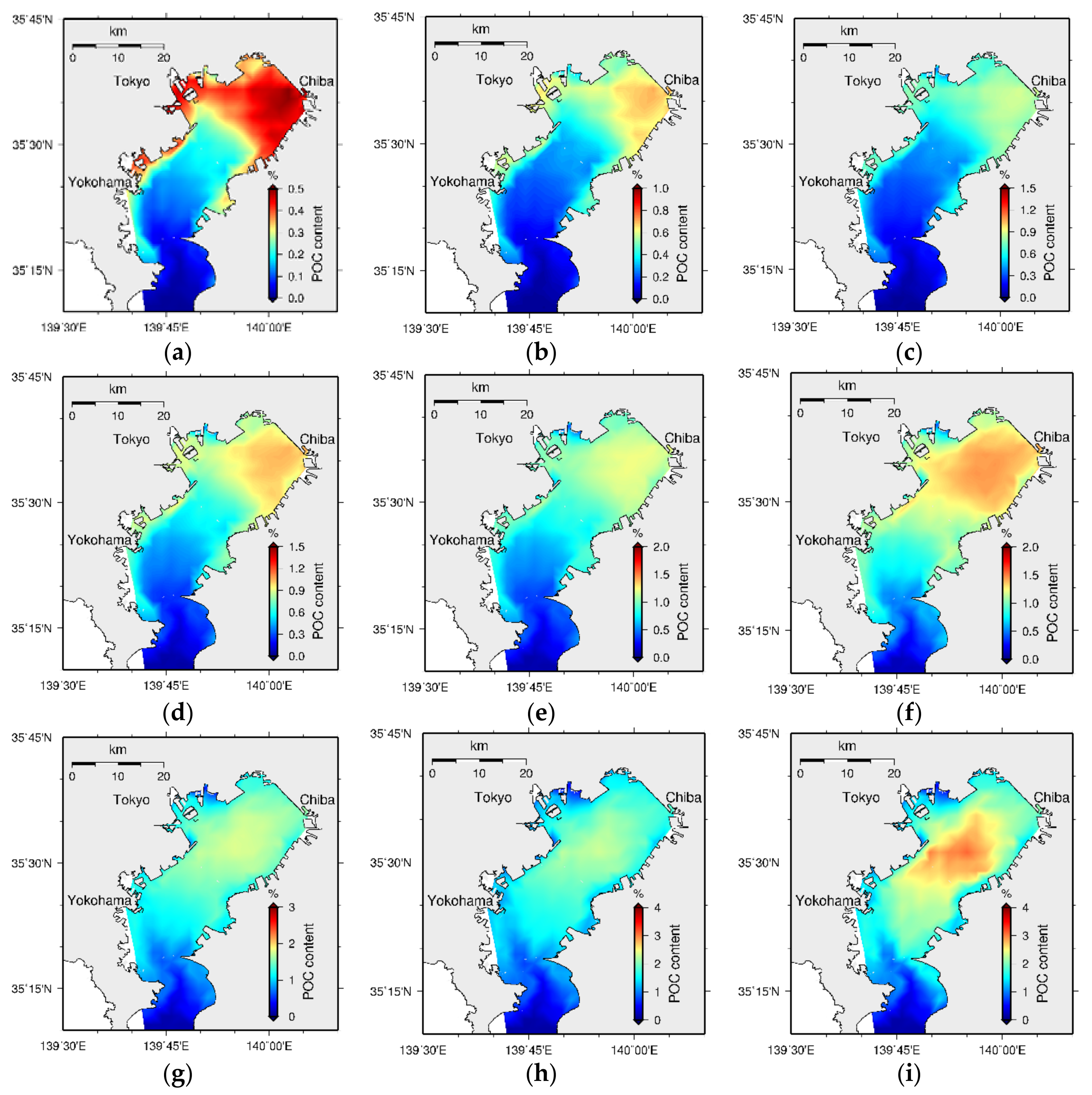
Tokyo Bay sediment bed formation with the accumulation of organic and inorganic particulate material over a 200-year period is shown in Figure 29. According to the results, high POCC initially appears at the head of the bay and moves towards the central part of the bay over time. This suggests that the accumulated particulate matter at the head of the bay undergoes erosion, moves towards the central part of the bay over time owing to some physical influence, and settles down again causing the highest pollution at its central part. Figure 30 shows a schematic diagram of the movement of particles, assuming a simplified bay structure.

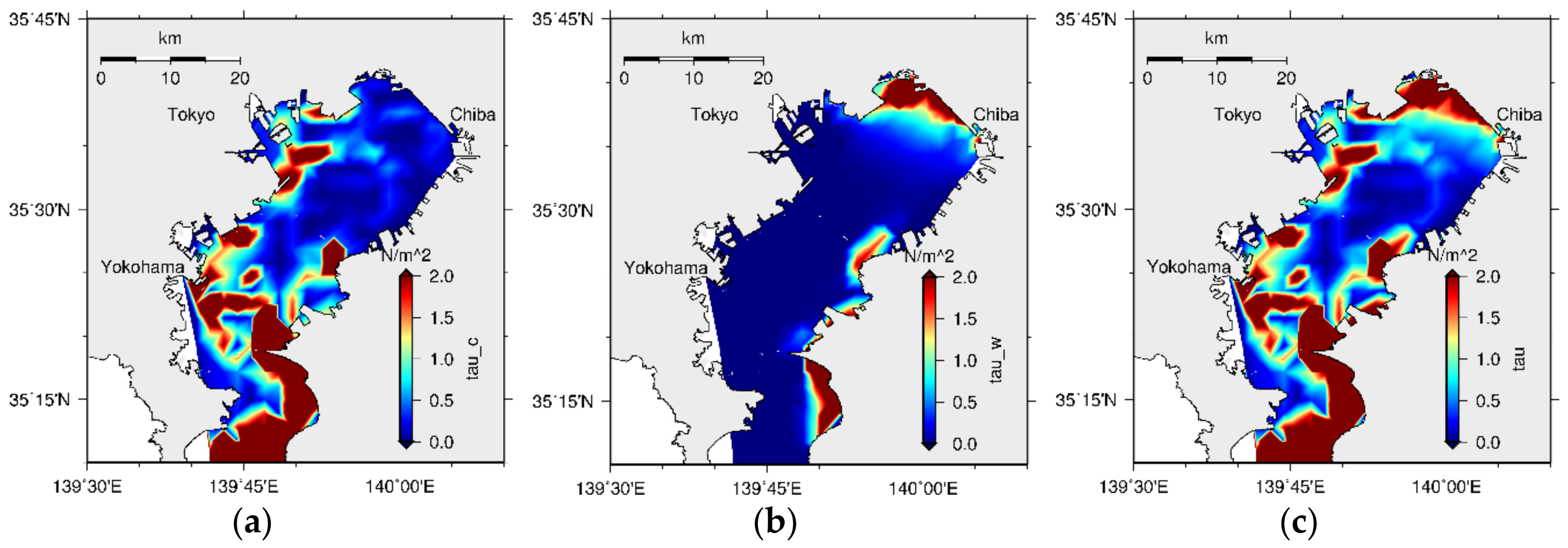
Initial bed formation can be discussed by considering the bathymetry distribution and silt accumulation in the bay. At the head of the bay, because the depth is shallower and the supply of silt from the rivers is comparatively low (the accumulation of silt becomes lower), the initial POCC becomes comparatively the highest. Deposition or erosion of particulate material is controlled by BSS, critical BSS on settling, and critical BSS on deposition. It has been modeled that when the BSS is lower than the critical BSS on deposition, resultant deposition occurs [40], and when the BSS is greater than the critical BSS on erosion, resultant erosion occurs [5]. The BSS distribution in the bay (Figure 31c) shows larger BSS at the head of the bay, and this has resulted in erosion at this part. These eroded sediment particles re-suspend at the bottom of the water column until they reach the condition to deposit again on the top of the sediment bed. However, if these particles move to another place within the water mass, the previously eroded particles may deposit at another location on the sediment surface. As a result, the area with high organic content sediment can be moved from one place to another. Hence, the water circulation within the bay is critical for analyzing the spatial distribution of sediment pollution in Tokyo Bay.

Water circulation owing to coastal upwelling in Tokyo Bay has been analyzed by many researchers based on field observations [66], laboratory experiments [67], numerical simulations [68], and analytical solutions [69]. Coastal upwelling in Tokyo Bay has resulted from frequent blowing of northeastern wind on the water surface. Matsuyama [68] and Zue and Isobe [69] have concluded that wind-induced coastal upwelling occurs at the northeast coast of Tokyo Bay. The movement of the surface water mass towards the mouth of the bay has caused upwelling of the bottom water mass to the surface at the head of the bay. This mechanism is influenced by the stable water stratification, especially during summer and autumn.

However, the final stable morphology of the bay, which shows the highest organic content towards its central part, has a strong relationship with the BSS distribution in the model. The BSS was modeled as a combination of CBSS and WBSS and, according to the model, CBSS is the highest at the bay mouth while the WBSS is the highest at the head of the bay, as shown in Figure 31. Hence, WBSS is responsible for the erosion at the head of the bay and thereby the movement of the organic rich area towards its central part. The results of the sensitivity analysis have confirmed that a kind of balance between the CBSS and WBSS keeps the Tokyo Bay sediment pollution at the central area.

This mechanism shows that WBSS is critical for a stable morphology in Tokyo Bay and confirms the previous research conclusions that wave generated shear stresses constitute the main mechanism responsible for sediment erosion and sediment export to salt marshes and to the ocean in shallow basins [70,71]. Moreover, numerical model experiments over morphologically different estuaries have also confirmed that waves are far more efficient than tides for eroding shallow areas [72], and small, locally generated waves that exert BSS have the potential to become a significant component of the sediment transport in shallow water areas [73]. Although the combined wave and current induced BSS change the estuary morphology, the relative contribution of the wave events in shaping the long-term morphological evolution in estuaries needs to be analyzed in detail [74].

6. Conclusions

Through a comprehensive model development strategy, an integrated, layer-resolved, process-based, sediment–water coupled, long-term robust, 3D estuarine ecosystem model—including realistic sedimentary and pelagic processes—was developed by this study. The model has been applied to Tokyo Bay and validated with available data. The model was computationally robust for long-term simulations and computed model results for 200 years have been used for the analysis. The computation was initiated with totally inorganic sediment to avoid the difficulties to obtain actual sediment data, and the expected states of water and sediment quality were obtained after long-term computation. The model was basically consistent with both the vertical distributions of water quality and spatial distributions of sediment quality. Reproducibility of the spatial distribution of organic rich sediment regardless of initial conditions has confirmed the robustness of the adopted modeling approach.

Sediment bed formation during 200 years has been analyzed during this study. Long-term model results have shown that high POCC, which starts at the head of the bay, moves towards the central part over time. Even though the mechanism for this sediment transport has to be analyzed in detail in future studies, it has shown some relationship with the BSS distribution. WBSS has become critical for erosion at the head of the bay and thereby for the transport of sediment towards its central part. However, the final stable morphology is decided by the balance between CBSS and WBSS.

This novel modeling approach, with the simplest sedimentary initial conditions and realistic sedimentary and pelagic processes, provides a great tool for long-term ecosystem modeling in future studies. The model forcing for long-term computation has been assumed constant during this study, and it is expected that the model will be applied with actual long-term meteorological data for predictions in future studies.

References

- Wild-Allen, K.; Skerratt, J.; Whitehead, J.; Rizwi, F.; Parslow, J. Mechanisms driving estuarine water quality: A 3D biogeochemical model for informed management. Estuar. Coast. Shelf Sci. 2013, 135, 33–45. [Google Scholar] [CrossRef]
- Weinberger, S.; Vetter, M. Using the hydrodynamic model DYRESM based on results of a regional climate model to estimate water temperature changes at Lake Ammersee. Ecol. Model. 2012, 244, 38–48. [Google Scholar] [CrossRef]
- Elhakeem, A.; Elshorbagy, W.; Bleninger, T. Long-term hydrodynamic modeling of the Arabian Gulf. Mar. Pollut. Bull. 2015, 94, 19–36. [Google Scholar] [CrossRef] [PubMed]
- Henderson, A.; Gamito, S.; Karakassis, I.; Pederson, P.; Smaal, A. Use of hydrodynamic and benthic models for managing environmental impacts of marine aquaculture. J. Appl. Ichthyol. 2001, 17, 163–172. [Google Scholar] [CrossRef]
- Rasmeemasmuang, T.; Sasaki, J. Modeling of mud accumulation and bed characteristics in Tokyo Bay. Coast. Eng. J. 2008, 50, 277–307. [Google Scholar] [CrossRef]
- Sohma, A.; Sekiguchi, Y.; Kuwae, T.; Nakamura, Y. A benthic–pelagic coupled ecosystem model to estimate the hypoxic estuary including tidal flat—Model description and validation of seasonal/daily dynamics. Ecol. Model. 2008, 215, 10–39. [Google Scholar] [CrossRef]
- De Mora, L.; Butenschön, M.; Allen, J.I. The assessment of a global marine ecosystem model on the basis of emergent properties and ecosystem function: A case study with ERSEM. Geosci. Model Dev. 2016, 9, 59–76. [Google Scholar] [CrossRef]
- Doney, S.C. Major challenges confronting marine biogeochemical modeling. Glob. Biogeochem. Cycles 1999, 13, 705–714. [Google Scholar] [CrossRef]
- Arhonditsis, G.B.; Brett, M.T. Evaluation of the current state of mechanistic aquatic biogeochemical modeling. Mar. Ecol. Prog. Ser. 2004, 271, 13–26. [Google Scholar] [CrossRef]
- Cerco, C.F.; Thomas, C. Three-dimensional eutrophication model of Chesapeake Bay. J. Environ. Eng. 1993, 119, 1006–1025. [Google Scholar] [CrossRef]
- Proctor, R.; Holt, J.T.; Allen, J.I.; Blackford, J. Nutrient fluxes and budgets for the North West European Shelf from a three-dimensional model. Sci. Total Environ. 2003, 314–316, 769–785. [Google Scholar] [CrossRef]
- Fennel, K.; Wilkin, J.; Levin, J.; Moisan, J.; O’Reilly, J.; Haidvogel, D. Nitrogen cycling in the Middle Atlantic Bight: Results from a three-dimensional model and implications for the North Atlantic nitrogen budget. Glob. Biogeochem. Cycles 2006, 20, GB3007. [Google Scholar] [CrossRef]
- Smits, J.G.C.; van Beek, J.K.L. ECO: A generic eutrophication model including comprehensive sediment–water interaction. PLoS ONE 2013, 8, 25. [Google Scholar] [CrossRef] [PubMed]
- Holstein, J.M.; Wirtz, K.W. Sensitivity analysis of nitrogen and carbon cycling in marine sediments. Estuar. Coast. Shelf Sci. 2009, 82, 632–644. [Google Scholar] [CrossRef] [Green Version]
- Soetaert, K.; Herman, P.M.J.; Middelburg, J.J. A model of early diagenetic processes from the shelf to abyssal depths. Geochim. Cosmochim. Acta 1996, 60, 1019–1040. [Google Scholar] [CrossRef]
- Krumins, V.; Gehlen, M.; Arndt, S.; Van Cappellen, P.; Regnier, P. Dissolved inorganic carbon and alkalinity fluxes from coastal marine sediments: Model estimates for different shelf environments and sensitivity to global change. Biogeosciences 2013, 10, 371–398. [Google Scholar] [CrossRef]
- Capet, A.; Meysman, F.J.R.; Akoumianaki, I.; Soetaert, K.; Grégoire, M. Integrating sediment biogeochemistry into 3D oceanic models: A study of benthic–pelagic coupling in the Black Sea. Ocean Model. 2016, 101, 83–100. [Google Scholar] [CrossRef]
- Mussap, G.; Zavatarelli, M. A numerical study of the benthic–pelagic coupling in a shallow shelf sea (Gulf of Trieste). Reg. Stud. Mar. Sci. 2017, 9, 24–34. [Google Scholar] [CrossRef]
- DiToro, D.M. Sediment Flux Modeling, 1st ed.; John Wiley & Sons, Inc.: New York, NY, USA, 2001; 656p, ISBN 978-0-471-13535-7. [Google Scholar]
- Ji, Z.-G. Hydrodynamics and Water Quality: Modeling Rivers, Lakes, and Estuaries; John Wiley & Sons, Inc.: New York, NY, USA, 2007; 704p, ISBN 9780470135433. [Google Scholar]
- Mann, K.H.; Lazier, J.R.N. Dynamics of Marine Ecosystems: Biological-Physical Interactions in the Oceans, 3rd ed.; John Wiley & Sons, Inc.: New York, NY, USA, 2013; 512p, ISBN 978-1-118-68791-8. [Google Scholar]
- Søndergaard, M.; Jensen, J.P.; Jeppesen, E. Role of sediment and internal loading of phosphorus in shallow lakes. Hydrobiologia 2003, 506–509, 135–145. [Google Scholar] [CrossRef]
- Burdige, D.J. 5.09—Estuarine and Coastal Sediments—Coupled Biogeochemical Cycling; Treatise on Estuarine and Coastal Science; Academic Press: Waltham, MA, USA, 2011; Volume 5, pp. 279–316. [Google Scholar]
- Soetaert, K.; Middelburg, J.J.; Herman, P.M.J.; Buis, K. On the coupling of benthic and pelagic biogeochemical models. Earth Sci. Rev. 2000, 51, 173–201. [Google Scholar] [CrossRef]
- Marcus, N.H.; Boero, F. Minireview: The importance of benthic–pelagic coupling and the forgotten role of life cycles in coastal aquatic systems. Limnol. Oceanogr. 1998, 43, 763–768. [Google Scholar] [CrossRef]
- Raffaelli, D.; Bell, E.; Weithoff, G.; Matsumoto, A.; Motta, J.J.C.; Kershaw, P.; Parker, R.; Parry, D.; Jones, M. The ups and downs of benthic ecology: Considerations of scale, heterogeneity and surveillance for benthic–pelagic coupling. J. Exp. Mar. Biol. Ecol. 2003, 285, 191–203. [Google Scholar] [CrossRef]
- Nakane, T.; Nakaka, K.; Bouman, H.; Platt, T. Environmental control of short-term variation in the plankton community of inner Tokyo Bay, Japan. Estuar. Coast. Shelf Sci. 2008, 78, 796–810. [Google Scholar] [CrossRef]
- Koibuchi, Y.; Isobe, M. Phytoplankton bloom mechanism in an area affected by eutrophication: Tokyo bay in spring 1999. Coast. Eng. J. 2007, 49, 461–479. [Google Scholar] [CrossRef]
- Han, M.S.; Furuya, K. Size and species-specific primary productivity and community structure of phytoplankton in Tokyo Bay. J. Plankton Res. 2000, 22, 1221–1235. [Google Scholar] [CrossRef]
- Han, M.S.; Furuya, K. Species-specific productivity of Skeletonema costatum (Bacillariophyceae) in the inner part of Tokyo Bay. Mar. Ecol. Prog. Ser. 1991, 79, 267–273. [Google Scholar] [CrossRef]
- Matsukawa, Y.; Sasaki, K. Nitrogen budget in Tokyo Bay with special reference to the low sedimentation to supply ratio. J. Oceanogr. Soc. Jpn. 1990, 46, 44–54. [Google Scholar] [CrossRef]
- Sasaki, J.; Kanayama, S.; Nakase, K.; Kino, S. Effective application of mechanical circulator for reducing hypoxia in an estuarine trench. Coast. Eng. J. 2009, 51, 309–339. [Google Scholar] [CrossRef]
- Fujiwara, T.; Yamada, Y. Inflow of oceanic water into Tokyo Bay and generation of a subsurface hypoxic water mass. J. Geophys. Res. Oceans 2002, 107, 1–13. [Google Scholar] [CrossRef]
- Heip, C.H.R.; Goosen, N.K.; Herman, P.M.J.; Kromkamp, J.C.; Middelburg, J.J.; Soetaert, K.E.R. Production and consumption of biological particles in temperate tidal estuaries. Oceanogr. Mar. Biol. Ann. Rev. 1995, 33, 1–149. [Google Scholar]
- Sasaki, J.; Isobe, M. Development of a long-term predictive model for baroclinic circulation and its application to blue tide phenomenon in Tokyo Bay. In Proceedings of the 27th International Conference on Coastal Engineering (ICCE), Sydney, Australia, 16–21 July 2000. [Google Scholar]
- Achiari, H.; Sasaki, J. Numerical analysis of wind-wave climate change and spatial distribution of bottom sediment properties in Sanbanze Shallows of Tokyo Bay. J. Coast. Res. 2007, SI50, 343–347. [Google Scholar]
- Orton, T.G.; Lark, R.M.; Sasaki, J. Using Geostatistics to analyze prediction errors from a simulation model of sediment particle sizes across Tokyo Bay. J. Coast. Res. 2013, 29, 141–156. [Google Scholar] [CrossRef]
- Okada, T.; Furukawa, K. Mapping sediment condition and benthos of shoreward area in Tokyo Bay. Annu. Coast. Eng. J. JSCE 2005, 52, 1431–1435. [Google Scholar]
- Okada, T.; Furukawa, K. Mapping sediment conditions of shoreward area in Tokyo Bay using echo features. Proc. Civ. Eng. Ocean 2005, 21, 749–754. [Google Scholar] [CrossRef]
- Attari, M.J.; Sasaki, J. An enhanced numerical model for material cycling and dissolved oxygen dynamics in Tokyo Bay, Japan. In Proceedings of the International Conference on Estuarine and Coastal Modeling, St. Augustine, FL, USA, 7–9 November 2011. [Google Scholar]
- Amunugama, A.A.W.R.R.M.K.; Sasaki, J.; Nakamura, Y.; Suzuki, T. Development of a benthic–pelagic coupled model for reproducing water quality in Tokyo Bay. J. Jpn. Soc. Civ. Eng. Ser. B3 Ocean Eng. 2015, 71, I_886–I_891. [Google Scholar]
- Amunugama, A.A.W.R.R.M.K.; Sasaki, J.; Nakamura, Y.; Suzuki, T. Spatial distribution of sediment quality in Tokyo Bay through benthic–pelagic coupled modeling approach. J. Jpn. Soc. Civ. Eng. Ser. B2 Coast. Eng. 2015, 71, I_1399–I_1404. [Google Scholar] [CrossRef]
- Koibuchi, Y.; Ogura, H.; Ando, H.; Gomyo, M.; Sasaki, J.; Isobe, M. Observation of annual cycle of nutrients in the inner part of Tokyo Bay. Proc. Coastal Eng. JSCE 2000, 47, 1066–1070. [Google Scholar]
- Sasaki, J.; Isobe, M. Development of a long-term predictive model of water quality in Tokyo Bay. In Proceedings of the 6th Conference on Estuarine and Coastal Modeling, ASCE, New Orleans, FL, USA, 1999; pp. 564–580. [Google Scholar]
- Patankar, S.V. Numerical Heat Transfer and Fluid Flow; McGraw-Hill Inc.: New York, NY, USA, 1980; 200p, ISBN 9780070487406. [Google Scholar]
- US Army Corps of Engineers. Shore Protection Manual, 4th ed.; Dept. of the Army, Waterways Experiment Station, Corps of Engineers, Coastal Engineering Research Center, Govt. Printing Office: Washington, DC, USA, 1984; 337p.
- Hasselmann, K.; Sell, W.; Ross, D.B.; Müller, P. A Parametric Wave Prediction Model. J. Phys. Oceanogr. 1976, 6, 200–228. [Google Scholar] [CrossRef]
- Bretschneider, C.L.; Reid, R. Change in wave height due to bottom friction, percolation and refraction. In Proceedings of the 34th Annual Meeting of American Geophisical Union, San Francisco, CA, USA, 14–18 December 2009. [Google Scholar]
- Putnam, J.A. Loss of wave energy due to percolation in a permeable sea bottom. EOS Trans. Am. Geophys. Union 1949, 30, 349–356. [Google Scholar] [CrossRef]
- Putnam, J.A.; Johson, J.W. The dissipation of wave energy by bottom friction. EOS Trans. Am. Geophys. Union 1949, 30, 67–74. [Google Scholar] [CrossRef]
- Van Rijn, L.C. Principles of Sediment Transport in Rivers, Estuaries and Coastal Seas; Aqua Publications: Blokzijl, The Netherland, 1993; Volume 1006, 715p, ISBN 90-800356-2-9. [Google Scholar]
- Gerritsen, H.; Vos, R.J.; van der Kaaij, T.; Lane, A.; Boon, J.G. Suspended sediment modelling in a shelf sea (North Sea). Coast. Eng. 2000, 41, 317–352. [Google Scholar] [CrossRef]
- Muller, A.C.; Muller, D.L. Forecasting future estuarine hypoxia using a wavelet based neural network model. Ocean Model. 2015, 96, 314–323. [Google Scholar] [CrossRef]
- Pan, C.W.; Chuang, Y.L.; Chou, L.S.; Chen, M.H.; Lin, H.J. Factors governing phytoplankton biomass and production in tropical estuaries of western Taiwan. Cont. Shelf Res. 2016, 118, 88–99. [Google Scholar] [CrossRef]
- Chai, C.; Jiang, T.; Cen, J.; Ge, W.; Lu, S. Phytoplankton pigments and functional community structure in relation to environmental factors in the Pearl River Estuary. Oceanologia 2016, 58, 201–211. [Google Scholar] [CrossRef]
- Agawin, N.S.R.; Duarte, C.M.; Agustí, S. Nutrient and temperature control of the contribution of picoplankton to phytoplankton biomass and production. Limnol. Oceanogr. 2000, 45, 591–600. [Google Scholar] [CrossRef]
- Riegman, R.; Kuipers, B.R.; Noordeloos, A.A.M.; Witte, H.J. Size-differential control of phytoplankton and the structure of plankton communities. Neth. J. Sea Res. 1993, 31, 255–265. [Google Scholar] [CrossRef]
- Fennel, W.; Neumann, T. Introduction to the Modelling of Marine Ecosystems; Halpern, D., Ed.; Elsevier: New York, NY, USA, 2004; Volume 72, 297p, ISBN 978-0444517029. [Google Scholar]
- Pennock, J.R. Chlorophyll distributions in the Delaware estuary: Regulation by light-limitation. Estuar. Coast. Shelf Sci. 1985, 21, 711–725. [Google Scholar] [CrossRef]
- Cote, B.; Platt, T. Day-to-day variations in the spring-summer photosynthetic parameters of coastal marine phytoplankton. Limnol. Oceanogr. 1983, 28, 320–344. [Google Scholar] [CrossRef]
- Walsh, J.J.; Whitledg, T.E.; Barvenik, F.W.; Wirick, C.D.; Howe, S.O. Wind events and food chain dynamics within the New York Bight. Limnol. Oceanogr. 1978, 23, 659–683. [Google Scholar] [CrossRef]
- Bouman, H.A.; Nakane, T.; Oka, K.; Nakata, K.; Kunta, K.; Sathyendranath, S.; Platt, T. Environmental controls on phytoplankton production in coastal ecosystems: A case study from Tokyo Bay. Estuar. Coast. Shelf Sci. 2010, 87, 63–72. [Google Scholar] [CrossRef]
- Harrison, W.G.; Platt, T. Photosynthesis-irradiance relationships in polar and temperate phytoplankton populations. Polar Biol. 1986, 5, 153–164. [Google Scholar] [CrossRef]
- Goldman, J.C.; Carpenter, E.J. A kinetic approach to the effect of temperature on algal growth. Limnol. Oceanogr. 1974, 19, 756–766. [Google Scholar] [CrossRef]
- Sasaki, J.; Koibuchi, Y.; Isobe, M. Realistic numerical simulation of water quality and ecosystems in Tokyo Bay. In Proceedings of the Third Joint Meeting of the Coastal Environmental Science and Technology Panel of the United States-Japan Cooperative Program in Natural Resources, Yokohama, Japan, 16–19 July 2002; pp. 143–157. [Google Scholar]
- Otsubo, K.; Harashima, A.; Miyazaki, T.; Yasuoka, Y.; Muraoka, K. Field survey and hydraulic study of ‘Aoshio’ in Tokyo Bay. Mar. Pollut. Bull. 1991, 23, 51–55. [Google Scholar] [CrossRef]
- Yoon, J.S.; Nakatsuji, K.; Muraoka, K. Experimental study on wind-driven stratified flow in enclosed water body. Proc. Hydraul. Eng. 1993, 37, 285–292. [Google Scholar] [CrossRef]
- Matsuyama, M. Numerical experiment in Tokyo Bay: In relating to ‘Aoshio’. Bull. Coast. Oceangr. 1990, 28, 63–74. [Google Scholar]
- Zhu, Z.; Isobe, M. Criteria for the occurrence of wind-driven coastal upwelling associated with ‘Aoshio’ on the southeast shore of Tokyo Bay. J. Oceanogr. 2012, 68, 561–574. [Google Scholar] [CrossRef]
- Fagherazzi, S.; Wiberg, P.L. Importance of wind conditions, fetch, and water levels on wave-generated shear stresses in shallow intertidal basins. J. Geophys. Res. Earth Surf. 2009, 114, F03022. [Google Scholar] [CrossRef]
- Liu, G.; Wu, J.; Wang, Y. Near-bed sediment transport in a heavily modified coastal plain estuary. Int. J. Sediment Res. 2014, 29, 232–245. [Google Scholar] [CrossRef]
- Hunt, S.; Bryan, K.R.; Mullarney, J.C. The influence of wind and waves on the existence of stable intertidal morphology in meso-tidal estuaries. Geomorphology 2015, 228, 158–174. [Google Scholar] [CrossRef]
- Green, M.O. Very small waves and associated sediment resuspension on an estuarine intertidal flat. Estuar. Coast. Shelf Sci. 2011, 93, 449–459. [Google Scholar] [CrossRef]
- Hunt, S.; Bryan, K.R.; Mullarney, J.C. The effect of wind waves on spring-neap variations in sediment transport in two meso-tidal estuarine basins with contrasting fetch. Geomorphology 2017, 280, 76–88. [Google Scholar] [CrossRef]
- Horiguchi, F. Numerical simulations of seasonal cycle of Tokyo Bay using an ecosystem model. J. Adv. Mar. Sci. Technol. Soc. 2001, 12, 1–30. [Google Scholar]
- Rounds, S.; Wood, T.M.; Lynch, D.D. Modeling Discharge, Temperature, and Water Quality in the Tualatin River, Oregon; U.S. Department of the Interior, U.S. Geological Survey: Reston, VA, USA, 1999.
- Paasche, E. Silicon and the ecology of marine plankton diatoms. II. Silicate-uptake kinetics in five diatom species. Mar. Biol. 1973, 19, 262–269. [Google Scholar] [CrossRef]
- Bowie, G.L.; Mills, W.B.; Porcella, D.B.; Campbell, C.L.; Pagenkopf, J.R.; Rupp, G.L.; Johnson, K.M.; Chan, P.W.H.; Gherini, S.A. Rates, Constants, and Kinetics Formulations in Surface Water Quality Modeling, 2nd ed.; United States Environmental Protection Agency, Office of Research and Development, Environmental Research Laboratory: Athens, GA, USA, 1985; 105p.
- Baretta, J.; Ruardij, P. Tidal Flat Estuaries; Springer: Berlin/Heidelberg, Germany, 1988; Volume 71, 281p, ISBN 978-3-642-73753-4. [Google Scholar]
Figure 1.
Map of Tokyo Bay with its rivers, sewer inputs, and collected data locations.
Figure 2.
Framework of the integrated biogeochemical model.
Figure 3.
Schematic diagram of pelagic biogeochemical processes and benthic–pelagic coupling.
Figure 4.
Schematic diagram of benthic biogeochemical processes and benthic–pelagic coupling.
Figure 5.
Schematic diagram for the effect of POCC on layer thickness [42].
Figure 6.
Boundary flux in (a) water column and (b) sediment column.
Figure 7.
(a) 2D control volume in a vertical section and (b) boundary flux at sediment–water interface.
Figure 8.
Relationship between observed porosity and POCC in Tokyo Bay [41].
Figure 9.
Locations of the river discharges and sewage outfall point sources to Tokyo Bay.
Figure 10.
Meteorological conditions during a one-year period: (a) Rainfall, (b) air temperature, (c) solar radiation, (d) air pressure, (e) vapor pressure, (f) relative humidity, (g) cloud cover, and (h) wind vector.
Figure 11.
Measured and simulated salinity [43].
Figure 12.
Measured and simulated values of surface and bottom salinity at (a) CLH, (b) KSB, and (c) TLH [43].
Figure 13.
Measured and simulated temperature [43].
Figure 14.
Measured and simulated values of surface and bottom temperature at (a) CLH, (b) KSB, and (c) TLH [43].
Figure 15.
Measured and simulated chlorophyll a [43].
Figure 16.
Measured and simulated values of surface and bottom chlorophyll a at (a) CLH, (b) KSB, and (c) TLH [43].
Figure 17.
Measured and simulated DO [43].
Figure 18.
Measured and simulated values of surface and bottom DO at (a) CLH, (b) KSB, and (c) TLH [43].
Figure 19.
Measured and simulated ammonia [43].
Figure 20.
Measured and simulated values of surface and bottom ammonia at (a) CLH, (b) KSB, and (c) TLH [43].
Figure 21.
Measured and simulated phosphate [43].
Figure 22.
Measured and simulated values of surface and bottom phosphate at (a) CLH, (b) KSB, and (c) TLH [43].
Figure 23.
Measured and simulated values of surface and bottom nitrate (a) CLH, (b) KSB, and (c) TLH [43].
Figure 24.
Measured and simulated nitrate [43].
Figure 25.
Measured and simulated silica [43].
Figure 26.
Measured and simulated values of surface and bottom silica at (a) CLH, (b) KSB, and (c) TLH [43].
Figure 27.
Spatial distribution of POCC in sediment: (a) observed (dots are sampling points) [39] and (b) simulated.
Figure 28.
Spatial distribution of WC in sediment: (a) observed (dots are sampling points) [39] and (b) simulated.
Figure 29.
Bed formation every 20-year time interval (a) 20-year (b) 40-year (c) 60-year (d) 80-year (e) 100-year (f) 120-year (g) 140-year (h) 160-year (i) 180-year, and (j) 200-year (note that the scales are different in each figure).
Figure 30.
Schematic diagram showing the movement of POC from the head to the central part of the bay: (a) initial high POCC at the head, (b) erosion due to BSS effect, and (c) effect of WBSS and CBSS to keep the highest POCC at the central area.Initially, the highest accumulation occurs at the head of the bay, as seen in (a), and the accumulated surface sediment is eroded and re-suspended owing to BSS (b). The re-suspended material can be moved to another location owing to physical processes within the bay. The final stable morphology is decided by the effects of WBSS and CBSS, suggesting possible higher accumulation of POCC towards the central part (c).
Figure 31.
Spatial distribution of (a) current induced, (b) wave induced, and (c) total bed shear stresses.