Fast Simulation of Large-Scale Floods Based on GPU Parallel Computing

Abstract

Computing speed is a significant issue of large-scale flood simulations for real-time response to disaster prevention and mitigation. Even today, most of the large-scale flood simulations are generally run on supercomputers due to the massive amounts of data and computations necessary. In this work, a two-dimensional shallow water model based on an unstructured Godunov-type finite volume scheme was proposed for flood simulation. To realize a fast simulation of large-scale floods on a personal computer, a Graphics Processing Unit (GPU)-based, high-performance computing method using the OpenACC application was adopted to parallelize the shallow water model. An unstructured data management method was presented to control the data transportation between the GPU and CPU (Central Processing Unit) with minimum overhead, and then both computation and data were offloaded from the CPU to the GPU, which exploited the computational capability of the GPU as much as possible. The parallel model was validated using various benchmarks and real-world case studies. The results demonstrate that speed-ups of up to one order of magnitude can be achieved in comparison with the serial model. The proposed parallel model provides a fast and reliable tool with which to quickly assess flood hazards in large-scale areas and, thus, has a bright application prospect for dynamic inundation risk identification and disaster assessment.

1. Introduction

Flooding due to dam-break, excessive rainfall, and storm surge is a serious threatening hazard that can cause significant casualties and economic losses. In recent years, the shallow water model has been widely researched and used for flood simulations [1,2,3,4,5,6]. Song et al. [1] proposed a robust and well-balanced finite volume model by using a new formulation of shallow water equations. Bi et al. [2] adopted adaptive Cartesian grids for the trade-off between model accuracy and efficiency. Wu et al. [3] presented a two-dimensional, well-balanced shallow water model for simulating flows over arbitrary topography with wetting and drying. Liu et al. [4] proposed a coupled 1D–2D hydrodynamic model for flood risk mapping. Rehman and Cho [5] proposed a robust method of slope source term treatment for modeling shallow-water flows and near-shore tsunami propagation. Kvocka et al. [6] determined a threshold value of the bottom slope for using the flood inundation model with shock-capturing algorithms. Those works have attracted much attention to the model accuracy and computational stability for wet/dry treatments over irregular topography.

Real-time flood control operations can reduce the social and economic loss caused by natural disasters [7]. To provide timely warning, which is very important for a real-time response to disaster prevention and mitigation, the large-scale floods should be simulated with a fast computing speed. Even today, most of the large-scale flood simulations are generally run on supercomputers due to the massive amounts of data and computations necessary. Sanders et al. [8] proposed a parallel shallow-water code, named ParBreZo, for high-resolution flood inundation modeling at the regional scale. Lai and Khan [9] adopted the message-passing interface (MPI) method to develop a parallel two-dimensional discontinuous Galerkin method for shallow-water flows. Since the multi-CPUs provided by supercomputers are relatively expensive, the more cost-effective computation platform based on a personal computer with a graphics processing unit (GPU) card could be used for fast simulation of large-scale floods, regarding the development that now one GPU card integrating thousands of computing cores can provide a powerful computational capability [10]. For example, Wang and Yang [11] adopted the GPU-based, high-performance-integrated hydrodynamic modelling system to simulate flood processes at the basin scale.

There are two main approaches for GPU parallelization, i.e., the CUDA (Compute Unified Device Architecture) programming language and the OpenACC application programming interface. The CUDA programming language, including CUDA C, CUDA Fortran, and OpenCL (Open Computing Language), favors low-level development, but has great flexibility in the parallel execution model, whereas the OpenACC application programming interface is a collection of runtime routines and compiler directives that use the FORTRAN or C/C++ languages to compile the specified code blocks of computational loops [12]. The OpenACC provided by the PGI compiler enables automatic code transplantation and the offloading of both massive amounts of data and computation from the CPU to the GPU. However, when using the CUDA programming language, both the parallel codes and execution parameters should be specified by the developer. Thus, it can be concluded that the OpenACC application programming interface is easier to use and has the advantage of better portability. Zhang et al. [13] evaluated three parallel methods, including OpenMP (Open MultiProcessing), MPI, and OpenACC, for the computation of a two-dimensional dam-break model using the explicit finite volume method. The Tesla K20c (Nvidia, CA, USA) with 2496 Nvidia CUDA cores was used for GPU computing. The computational area is 1997 km², and 337,084 quadrilateral unstructured meshes were used. The average grid length is 80 m. The results showed that the OpenACC parallel method using a Tesla K20c GPU card achieved a higher speedup ratio than that of the OpenMP and MPI parallel methods on a 32-core computer. Liang et al. [14] used the OpenCL language and then developed a GPU-accelerated hydrodynamic model for a rainfall-runoff process simulation. The Tesla K80 with 4992 Nvidia CUDA cores was used for GPU computing. The time consumption of the simulation for a 12-h flood event on 5 million computational cells at 5 m resolution was 2.5 h when using a single Tesla K80 GPU card (Nvidia, CA, USA). Thus, it can be concluded that a GPU-based personal computer can enable catchment-scale simulations at a very high spatial grid resolution and substantially improve the computational efficiency. GPU-accelerated models have also been used for the simulation of coastal ocean tides [15], waves [16], and dam-break floods [17], showing a noticeable speedup. Néelz and Pender [18] presented various benchmarks for the latest generation of 2D hydraulic modelling packages, including the MIKE21 FM model, TUFLOW, and so on. The results show that the MIKE21 FM model can be used for flood simulation.

In this work, a two-dimensional shallow water model based on an unstructured Godunov-type explicit finite volume scheme is proposed for flood simulation. The HLLC (Harten, Lax, vanLeer, Contact) solver is adopted for flux computation, and the flow states are updated by Hancock’s prediction-correction scheme. The main computational subroutines are presented as loops with data independence and natural parallelism. To realize fast simulation of large-scale floods on a personal computer, a graphics processing unit (GPU)-based high-performance computing method using the OpenACC application programming interface was adopted to parallelize the shallow water model in an incremental developing way with minimal recoding work. An unstructured data management method is presented to control the data transportation between the GPU and the CPU with minimal overhead, and then both computation and data are offloaded from the CPU to the GPU, which can exploit the computational capability of the GPU as much as possible. The parallel model is validated using various benchmarks and real-world case studies.

2. Methodologies

2.1. Hydrodynamic Model

2.1.1. Governing Equations

The 2D shallow water equations are used as the governing equations for the flood simulation, which are given in the following conservation form:

$$\frac{\partial U}{\partial t}+\frac{\partial E}{\partial x}+\frac{\partial G}{\partial y}=S$$

(1)

in which

$$U=\left[\begin{array}{c}h\\ hu\\ hv\end{array}\right],E=\left[\begin{array}{c}hu\\ h{u}^2+g(h^2-b^2)/2\\ huv\end{array}\right],G=\left[\begin{array}{c}hv\\ huv\\ h{v}^2+g(h^2-b^2)/2\end{array}\right],S=S_0+S_f=\left[\begin{array}{c}0\\ g(h+b)S_{0x}\\ g(h+b)S_{0y}\end{array}\right]+\left[\begin{array}{c}0\\ -gh{S}_{fx}\\ -gh{S}_{fy}\end{array}\right]$$

in which $h$ is the depth; $u$ and $v$ are the velocity in the $x$- and $y$-directions, $b$ is the bed elevation, $S_{0x}$ and $S_{0y}$ are the bed slopes in the $x$- and $y$-directions, $S_{0x}=-\partial b/\partial x$ and $S_{0y}=-\partial b/\partial y$, $g$ is the gravity acceleration, and $S_{fx}$ and $S_{fy}$ are the friction terms. The friction terms are estimated by Manning formulae [1]:

$$S_{fx}=\frac{n^{2}u\sqrt{u^2+v^2}}{h^{4/3}},S_{fy}=\frac{n^{2}v\sqrt{u^2+v^2}}{h^{4/3}}$$

(2)

in which n is the empirical Manning coefficient.

2.1.2. Numerical Method

One of the widely-used Godunov-type finite volume methods for solving the two-dimensional shallow water equations, named the MUSCL (Monotone Upstream Scheme for Conservation Law)-Hancock scheme, is adopted in this work. The computational grids are triangular. The processes of updating flow states are given as follows:

(1) Wet/dry classification for nodes and cells

Since flood simulations always involve a dry bed case, the computational cells and nodes should be classified for wet/dry front treatment. In this paper, a nodal water depth-based method is used for classification. When a nodal depth is greater than 10⁻³ m [4], the node would be classified as a wet-node; otherwise, the node would be classified as a dry-node. Based on the nodal wet/dry classification, a wet-cell is defined as that in which all three nodes of the cell are wetted; and if one or more nodes of a cell are dry, the cell is classified as a dry-cell. It can be concluded that the subroutine of wet/dry classification is a computational loop with data independence.

It should be noted that, in general, the threshold for wet and dry classification is non-sensitive to the final computational results of the maximum water depth and flow velocity. However, it would influence the time of arrival of the floods. For example, if we set the threshold to be an unreasonable value of 1 m, then the flood front propagation would be numerically hindered by the wet and dry classification, as the water depth must be higher than 1 m for flooding. However, if we set the threshold to be small enough, such as 10⁻³ m or 10⁻⁶ m, the threshold is non-sensitive to the final computational results, including the maximum water depth, flow velocity, the time of arrival of the floods, and so on.

(2) Gradient calculation for cells

To achieve higher-order accuracy, as well as computational stability, a hybrid method is adopted for gradient computation. If a cell is classified as dry, the gradients of the water level and velocities are set to zero. Otherwise, the unlimited gradient is computed based on values at centroids of three neighboring cells using the plane gradient calculation method. To preserve the TVD (total variation diminishing) property, the limit function used by Song et al. [1] is adopted for limited gradient calculations. It can be concluded that the subroutine of the gradient calculation is a computational loop with data independence.

(3) Prediction calculation for cells

The predictor results at the time step m + 1/2 are computed by using values of the water level, water depth, velocities, and their limited gradients at the basis time step m:

$${\eta }_i^{m+1/2}={{\eta }_i^m-\frac{\mathsf{\Delta }t}{2}(h\overline{{\partial }_x}u+h\overline{{\partial }_y}v+u\overline{{\partial }_x}h+v\overline{{\partial }_y}h)|}_i^m$$

(3)

$$u_i^{m+1/2}={\frac{1}{1+g{n}^2{h}^{-4/3}\sqrt{u^2+v^2}\mathsf{\Delta }t/2}[u-\frac{\mathsf{\Delta }t}{2}(u\overline{{\partial }_x}u+g\overline{{\partial }_x}\eta +v\overline{{\partial }_y}u)]|}_i^m$$

(4)

$$v_i^{m+1/2}={\frac{1}{1+g{n}^2{h}^{-4/3}\sqrt{u^2+v^2}\mathsf{\Delta }t/2}[v-\frac{\mathsf{\Delta }t}{2}(u\overline{{\partial }_x}v+g\overline{{\partial }_y}\eta +v\overline{{\partial }_y}v)]|}_i^m$$

(5)

in which the superscript m is the time step, $\eta$ is the water level, $\mathsf{\Delta }t$ is the computational time step, $\overline{\partial }$ denotes the limited gradient, and the subscript i is the element index. It can be concluded that the subroutine of the prediction calculation is a computational loop with data independence.

(4) Variable reconstruction for edges

If the cell is classified as a wet-cell, the linear interpolation method is used for variable reconstruction based on the limited gradient at the basis time step n and the predictor results. If the cell is classified as a dry-cell, the reconstructed face values of the velocities are extrapolated from centric values:

$$u_{i,k}^{\mathrm{Rec}}=u_i{v}_{i,k}^{\mathrm{Rec}}=v_i(k=1,2,3)$$

(6)

and the reconstructed water depth is given by

$$h_{i,k}^{\mathrm{Rec}}=\{\begin{array}{llll}0\hfill & \mathrm{if}\hfill & {\eta }_i\le b_{i,k}^{\min }\hfill & \\ \frac{{({\eta }_i-b_{i,k}^{\min })}^2}{2(b_{i,k}^{\max }-b_{i,k}^{\min })}\hfill & \mathrm{if}\hfill & b_{i,k}^{\min }<{\eta }_i\le b_{i,k}^{\max }\hfill & (k=1,2,3)\hfill \\ {\eta }_i-\frac{b_{i,k}^{\min }+b_{i,k}^{\max }}{2}\hfill & \mathrm{if}\hfill & {\eta }_i>b_{i,k}^{\max }\hfill & \end{array}$$

(7)

in which $b_{i,k}^{\min }$ and $b_{i,k}^{\max }$ are the minimum and maximum bed elevations of the two endpoints of edge $k$ in cell $C_i$. It can be concluded that the subroutine of variable reconstruction is a computational loop with data independence.

(5) Numerical flux calculations for edges

The numerical fluxes are computed by using the HLLC Riemann solver, which is given by

$$F(U_{\mathrm{L}},U_{\mathrm{R}})\cdot n=\{\begin{array}{ll}F(U_{\mathrm{L}})\cdot n\hfill & \mathrm{if}{s}_1\ge 0\hfill \\ F_{*\mathrm{L}}\hfill & \mathrm{if}{s}_1<0\le s_2\hfill \\ F_{*\mathrm{R}}\hfill & \mathrm{if}{s}_2<0<s_3\hfill \\ F(U_{\mathrm{R}})\cdot n\hfill & \mathrm{if}{s}_3\le 0\hfill \end{array}$$

(8)

in which n = (n_x, n_y)^T is the unit outward normal vector; $F(U_{\mathrm{L}})\cdot n$, $F_{*\mathrm{L}}$, $F_{*\mathrm{R}}$, and $F(U_{\mathrm{R}})\cdot n$ are computed by

$$F(U)\cdot n=\left[\begin{array}{c}h{u}_{\perp }\\ hu{u}_{\perp }+\frac{1}{2}g(h^2-b^2)n_x\\ hv{u}_{\perp }+\frac{1}{2}g(h^2-b^2)n_y\end{array}\right]$$

(9)

$$F_{*\mathrm{L}}=\left[\begin{array}{c}{(E_{\mathrm{HLL}})}^1\\ {(E_{\mathrm{HLL}})}^2{n}_x-u_{//,\mathrm{L}}{(E_{\mathrm{HLL}})}^1{n}_y\\ {(E_{\mathrm{HLL}})}^2{n}_y+u_{//,\mathrm{L}}{(E_{\mathrm{HLL}})}^1{n}_x\end{array}\right]$$

(10)

$$F_{*\mathrm{R}}=\left[\begin{array}{c}{(E_{\mathrm{HLL}})}^1\\ {(E_{\mathrm{HLL}})}^2{n}_x-u_{//,\mathrm{R}}{(E_{\mathrm{HLL}})}^1{n}_y\\ {(E_{\mathrm{HLL}})}^2{n}_y+u_{//,\mathrm{R}}{(E_{\mathrm{HLL}})}^1{n}_x\end{array}\right]$$

(11)

and $s_1,s_2,s_3$ are wave speeds, which are given by

$$s_1=\{\begin{array}{ll}\min (u_{\perp ,\mathrm{L}}-\sqrt{g{h}_{\mathrm{L}}},u_{\perp ,*}-\sqrt{g{h}_{*}})& \mathrm{if}{h}_{\mathrm{L}}>0\\ u_{\perp ,\mathrm{R}}-2\sqrt{g{h}_{\mathrm{R}}}& \mathrm{if}{h}_{\mathrm{L}}=0\end{array}$$

(12)

$$s_3=\{\begin{array}{ll}\max (u_{\perp ,\mathrm{R}}+\sqrt{g{h}_{\mathrm{R}}},u_{\perp ,*}+\sqrt{g{h}_{*}})& \mathrm{if}{h}_{\mathrm{R}}>0\\ u_{\perp ,\mathrm{L}}+2\sqrt{g{h}_{\mathrm{L}}}& \mathrm{if}{h}_{\mathrm{R}}=0\end{array}$$

(13)

$$s_2=\frac{s_1{h}_{\mathrm{R}}(u_{\perp ,\mathrm{R}}-s_3)-s_3{h}_{\mathrm{L}}(u_{\perp ,\mathrm{L}}-s_1)}{h_{\mathrm{R}}(u_{\perp ,\mathrm{R}}-s_3)-h_{\mathrm{L}}(u_{\perp ,\mathrm{L}}-s_1)}$$

(14)

in which $h_{*}$ and $u_{\perp ,*}$ are middle states estimation given by

$$h_{*}=\frac{1}{2}(h_{\mathrm{L}}+h_{\mathrm{R}})u_{\perp ,*}=\frac{\sqrt{h_{\mathrm{L}}}{u}_{\perp ,\mathrm{L}}+\sqrt{h_{\mathrm{R}}}{u}_{\perp ,\mathrm{R}}}{\sqrt{h_{\mathrm{L}}}+\sqrt{h_{\mathrm{R}}}}$$

(15)

and $u_{\perp }=u{n}_x+v{n}_y$, $u_{//}=-u{n}_y+v{n}_x$. ${(E_{\mathrm{HLL}})}^1$, and ${(E_{\mathrm{HLL}})}^2$ are the first two components of the normal flux $E_{\mathrm{HLL}}$, which is computed by using the HLL formula

$$E_{\mathrm{HLL}}=\frac{s_{3}E(T{U}_{\mathrm{L}})-s_{1}E(T{U}_{\mathrm{R}})+s_1{s}_3(T{U}_{\mathrm{R}}-T{U}_{\mathrm{L}})}{s_3-s_1}$$

(16)

It can be concluded that the subroutine of the numerical flux calculation is a computational loop with data independence.

(6) Bed slope term approximation for cells

The cell-centered bed slope term approximation method is adopted in this work:

$$S_{i,0x}=-{\displaystyle \underset{C_i}{\int }g(h+b)\frac{\partial b}{\partial x}\mathrm{d}\mathsf{\Omega }}=-g(h_i+b_i){\frac{\partial b}{\partial x}|}_i{\mathsf{\Omega }}_i$$

(17)

$$S_{i,0y}=-{\displaystyle \underset{C_i}{\int }g(h+b)\frac{\partial b}{\partial y}\mathrm{d}\mathsf{\Omega }}=-g(h_i+b_i){\frac{\partial b}{\partial y}|}_i{\mathsf{\Omega }}_i$$

(18)

in which $\mathsf{\Omega }$ is the cell area. It can be concluded that the subroutine of the bed slope term approximation is a computational loop with data independence.

(7) Correction calculation for cells

The flow states at the next time step n + 1 are calculated by

$$U_i^{m+1}=U_i^m-\frac{\mathsf{\Delta }t}{{\mathsf{\Omega }}_i}{\displaystyle \sum _{k=1}^3{F}_k\cdot n_k{L}_k}+\frac{\mathsf{\Delta }t}{{\mathsf{\Omega }}_i}{S}_i$$

(19)

in which $L$ is the edge length and $S_i$ is the source approximation. It can be concluded that the subroutine of the correction is a computational loop with data independence.

2.2. GPU Parallel Computing

The OpenACC application programming interface provided by the PGI compiler is a collection of runtime routines and compiler directives that use the Fortran or C/C++ language to compile the specified code blocks of computational loops. In shallow water models, the key to an OpenACC-based parallel implementation is that all the data and computationally-intensive work should be offloaded from the CPU to the GPU with minimal data transportation. The flood simulation is iterated over a series of computational time-steps, and all calculation subroutines in a time-step should be run in parallel on the GPU for high-performance computation.

As the finite volume scheme adopted in this work is explicit, the main computational subroutines described above are presented as loops with data independence and natural parallelism. Thus, in a computational time-step, the calculations for each cell or edge are numerically decoupled, and the computational loops can be executed in parallel by the GPU device. Therefore, OpenACC clauses can be directly added to the original serial model codes to realize GPU computation, accelerating the program in an incrementally-developing way with minimal recoding work. In this study, a GPU-based high-performance computing method using the OpenACC application is adopted to parallelize the shallow water model.

The most significant issue of GPU-based parallelization is the design of the calculation flow, which involves three steps: data input, numerical computing, and results output. Since the Peripheral Component Interface express (PCIe) bus used for data transportation between the CPU and the GPU is relatively time-consuming, all data should be offloaded from the CPU to the GPU at the initial stage, and then the massive amounts of data should be consecutively processed in the GPU device space. Figure 1 presents the computational flow diagram for the GPU-based parallel model, from which it can be seen that the role of the CPU is designed as a calculation flow controller, as well as an I/O interface for data files, and the intensive computational work and data are consecutively processed in the GPU device space. Moreover, the unstructured data management method described above can control the data transportation between the GPU and the CPU with minimal overhead and, thus, can exploit the computational capability of the GPU as much as possible. It should be noted that the program targeted by the OpenACC application programming interface is host (CPU)-directed execution with an attached accelerator device (GPU). In the serial model, the subroutines are sequentially called and executed by the CPU. However, in the GPU-based parallel model, the subroutines are sequentially called by the CPU, but each of the subroutines are executed in parallel on the GPU, since the computation is offloaded from the CPU to the GPU. It should be noted that the GPU-based parallelization approach presented in this paper is not suitable for implicit schemes, since the problem of data dependence is difficult to resolve.

3. Model Validations

3.1. Flooding a Disconnected Water Body

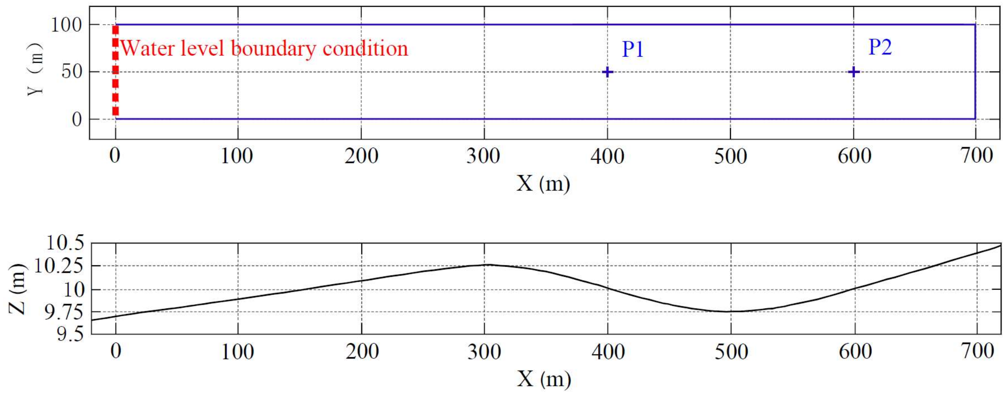
To assess basic capabilities, such as handling disconnected water bodies, the conservation of momentum, and the wetting and drying of floodplains, the test case used by Néelz and Pender [18] as a benchmark for 2D hydraulic modeling package testing is adopted in this work. The computational area consists of a 100 m wide, 700 m long domain with a longitudinal profile as illustrated in Figure 2. From the longitudinal profile, it can be seen that there is a pond located at x = 300–700 m. A water level boundary condition is applied upstream of the domain: in the first 1 h the water level rises from 9.7 m to a peak level of 10.35 m, and after a 10 h maintenance of the peak level for the depression on the right-hand side to fill up to a level of 10.35 m, the water level is lowered to 9.7 m in 1 h. The lateral and downstream boundaries are zero mass flux.

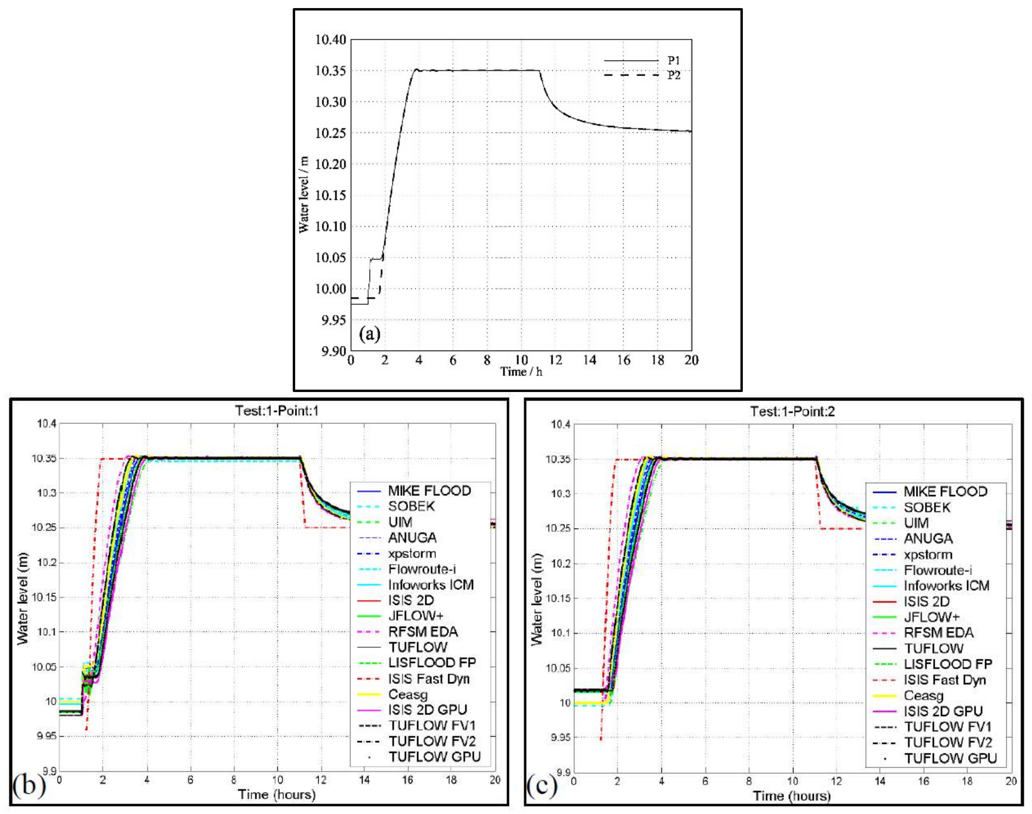
The initial water level is 9.7 m, and a uniform Manning coefficient of 0.03 is used in this case. The computed water levels at two points, P1 (400, 50) and P2 (600, 50), are presented in Figure 3a. Figure 3b,c shows the computed results of different models from Néelz and Pender [18]. The results show that the proposed model successfully simulates the sheet flow, of which the water depth is up to 0.05 m, at point 1, starting at t = 1 h and lasting for about 45 min until the water level in the pond reaches the ground elevation of P1. From Figure 3, it can be seen that the computed results of the proposed model match well with those of the MIKE model. Additionally, the water difference between P1 and P2 was negligible after t = 2 h. The final level elevation at P1 and P2 is 10.25 m, which equals the exact solution.

3.2. The Toce River Dam-Break Case with Overtopping

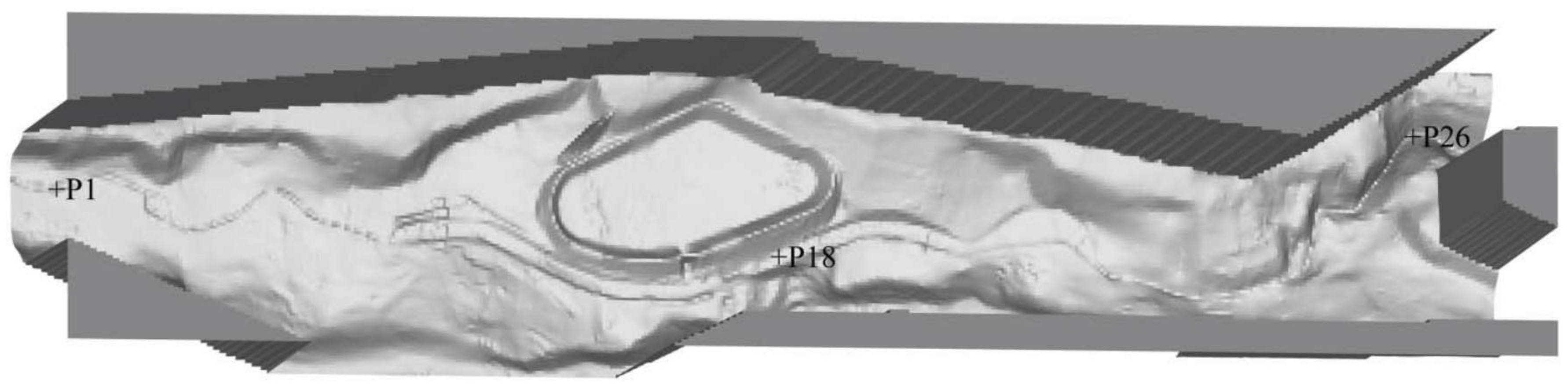
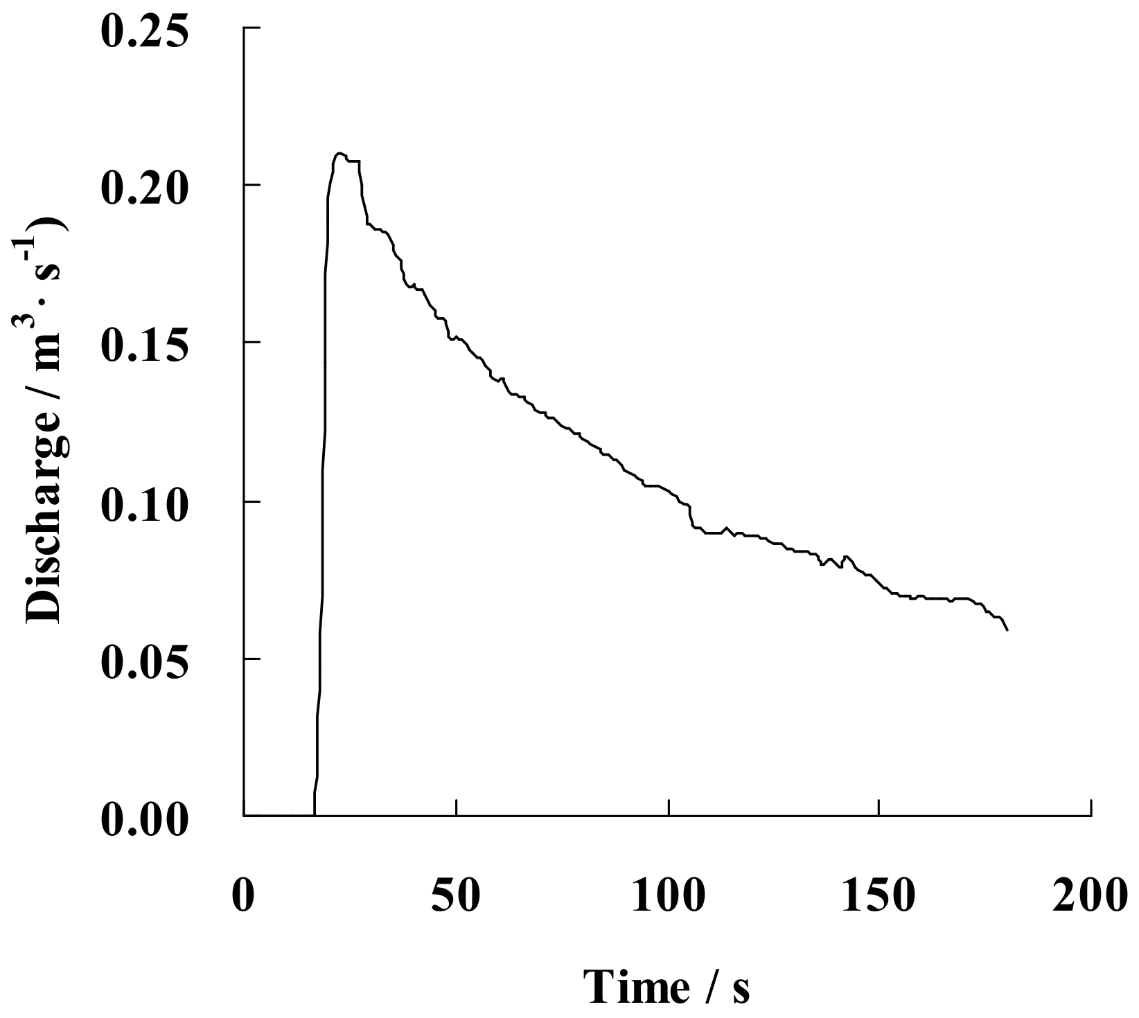
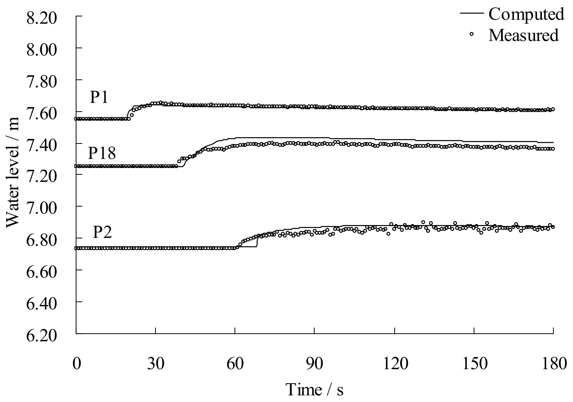
In this case, the parallel model is applied to simulate the dam break flood event in the physical model of the Toce River [19]. This case is used to test the shock-capturing property of the proposed model. Figure 4 shows the plan view of the topography of the Toce River physical model. The computational domain is approximately 50 × 11 m. Three selected gauges (P1, P18, and P26) along the main river axis are used for comparing the computed results with the measured data. A rectangular tank was located at the upstream end (i.e., the left end in Figure 4) of the physical model. The water level of the rectangular tank rose suddenly to model the dam-break flooding. In the middle of the domain there is an empty reservoir. The bank of the reservoir would be overtopped by river floods. In this case, discharge from the rectangular tank was used as an inflow boundary condition (Figure 5). The channel downstream of the tank is initially dry. The downstream boundary is an open flow condition. The lateral boundaries are zero mass flux. The value of the Manning coefficient is taken to be 0.016.

This case was simulated until t = 0.05 h. A comparison of the computed stage-time hydrographs with the measured data at three gauge points is shown in Figure 6. The results show that the proposed model is in agreement with the measured data.

4. Case Study: A Real Flood Simulation in the Wei River

4.1. Study Area

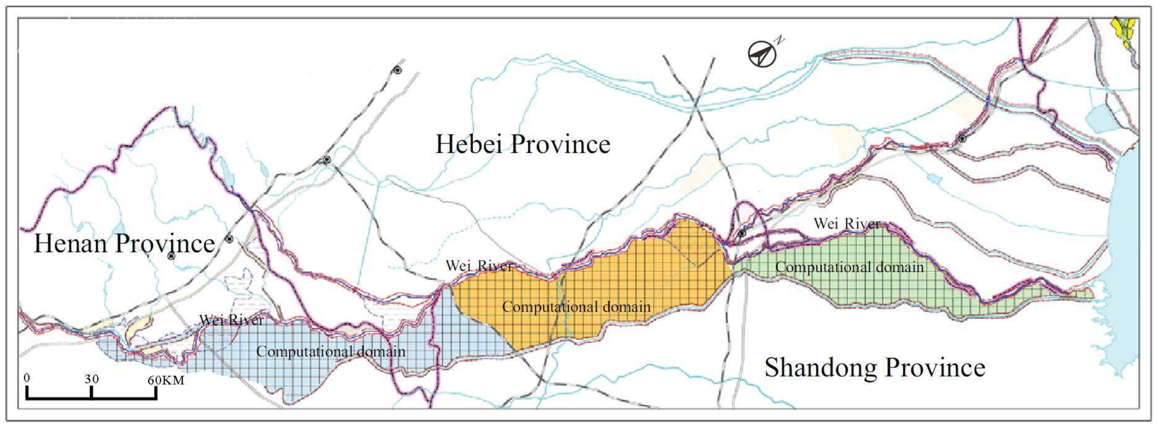
The Wei River Basin is located on the windward slope (i.e., east slope) of Taihang Mountain, so there are frequent and heavy rainstorms, leading to serious flood disasters in most years. From 1670 to 2005 there were 110 recorded great floods, and the flood disasters occurred, on average, once every three years. In August 1996, the economic loss due to flood was up to RMB 1.04 billion, and the flood inundation area was about 191 km². The flood control protection zone of the Wei River right bank involves Shandong, Hebei, and Henan provinces in China (Figure 7), and in Figure 7 the blocks of hatch pattern with different colors belong to different provinces. There are about 180 townships in the flood control protection zone. The study area is bounded by the left embankment of the Tuhaimajia River, the left embankment of the Majia River, the Bohai Estuary, the right embankment of the Zhangweixin River, the right embankment of the Weiyunhe Canal, and the right embankment of the Wei River. The total area is about 9503 km², which is a large-scale field and is time-consuming for flood simulation.

4.2. Computational Mesh

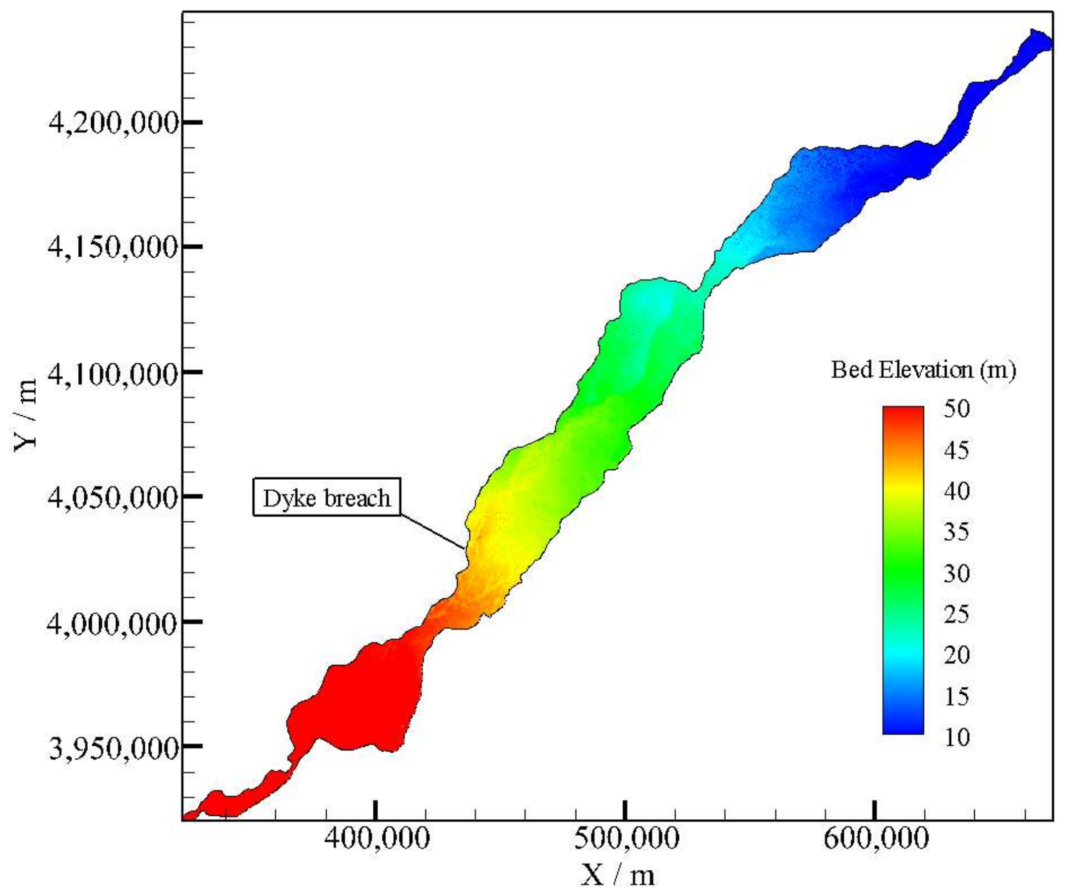
In this work, three grid division schemes with different resolutions are considered to test the performance of the parallel model. The first division is a basis of 179,296 triangular grids with average side-lengths varying form 50–250 m, and the average area of grids is 0.053 km². The other two divisions are refined, in turn, by evenly dividing one grid into four grids from the middle points of the edges, and the corresponding total triangular grid numbers are 717,184 and 2,868,736, respectively. For simplified expression, the three grid divisions are denoted as mesh-1, mesh-2, and mesh-3, respectively. Figure 8 shows the topography of the study area using Gauss-Kruger projection.

4.3. Dyke-Break Flood Simulation

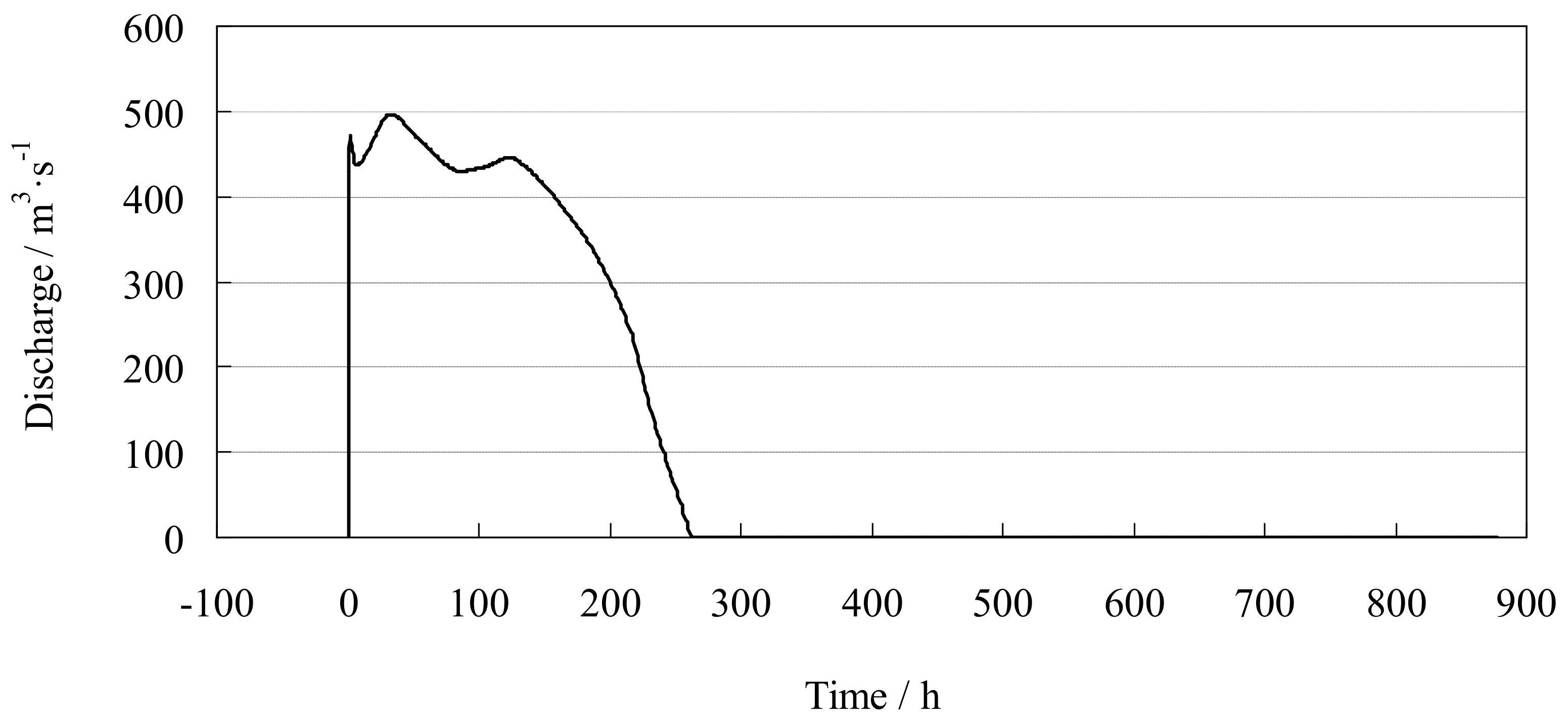
We consider a hypothetical dyke breach, and the position is shown in Figure 8. The discharge across the breach is shown in Figure 9, assuming the dyke breach occurred at time t = 0. The peak discharge is 496 m³/s, and the flooding duration time is about 263 h. To simulate the whole process of flooding and recession, the computation time is set to 878 h, and the discharge across the breach is 0 during time t = 264–878 h.

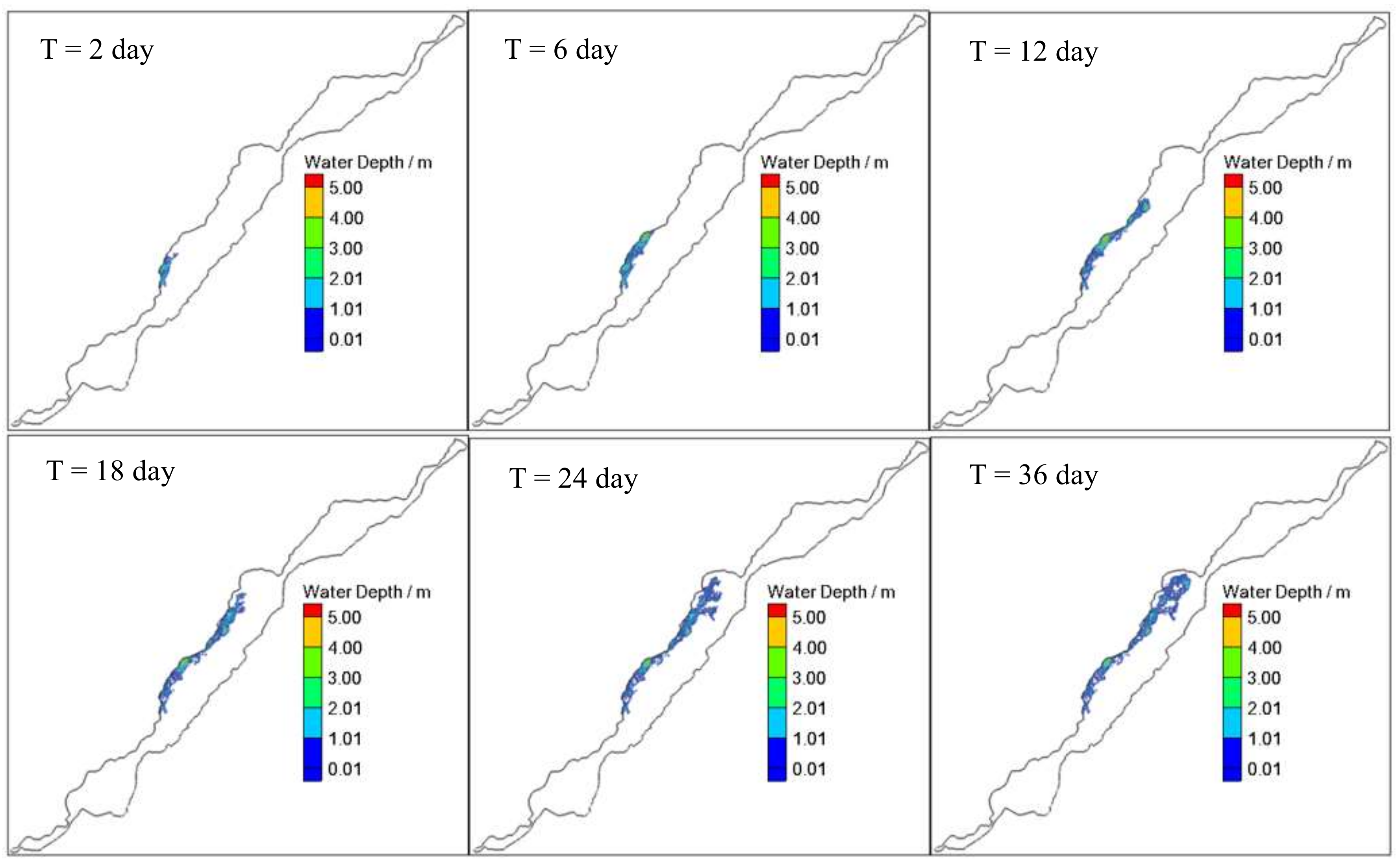
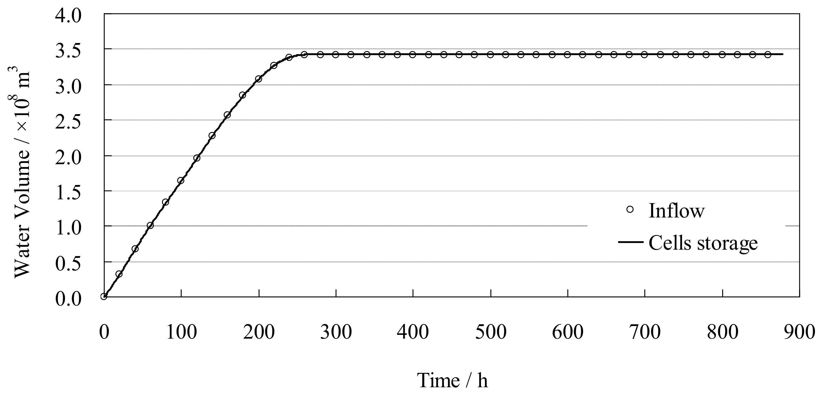
Figure 10 shows the distribution of the computed water depth at different times using mesh-1, from which it can be seen that the flood propagation is well simulated. Both the direction and extent of the flood propagation are consistent with the topography. Figure 11 shows the water volume of the inflow and the cells’ storage, from which it can be seen that the computed cells’ water storage equals the inflow water volume, validating the property of mass conservation of the proposed model.

Table 1. The test case of real flood simulation in the Wei River: the comparison of the final flooded area at different water depth intervals (km²).

Model	In All	Water Depth Intervals
		0.05–0.5 m	0.5–1 m	1–2 m	2–3 m	≥3 m
MIKE21 FM	864.26	370.35	234.5	200.34	50.14	8.93
The proposed model	856.28	364.62	241.19	193.46	47.03	9.98
Relative error (%)	−0.92%	−1.55%	2.85%	−3.43%	−6.20%	11.76%

gives the comparison of the final flooded area at different water depth intervals between the proposed model and the MIKE21 FM model. The results show that the total flooded area computed by the proposed model matches well with the MIKE21 FM model, and the differences at five water depth intervals are very small in the view of practical application. From Table 1, it can be seen that the absolute relative error increases with the increase of the water depth. The flooded area computed by the proposed model is larger than that of MIKE21 FM for water depth intervals of 0.5–1 m and ≥3 m, while the flooded area computed by the proposed model is smaller than that of MIKE21 FM for water depth intervals of 0.05–0.5 m, 1–2 m, and 2–3 m. These differences are produced by the model structure error. Since the real topography is very complex, the flooded area of higher water depth would have a more complicated flow pattern, which should introduce more numerical error between the proposed model and the MIKE21 FM model.

4.4. Parallel Performance Analysis

The parallel performance analyses of the flood simulation model are based on executions of the OpenACC-directed codes on the GPU, compared to the executions of serial codes on the CPU. In this work, we use an Intel Xeon CPU E5-2690 @ 3.0 GHz (Intel, CA, USA) for running the serial model and additionally adopt one Tesla K20 card for the parallel model. The GPU card has a Kepler GK110 GPU (Nvidia, CA, USA) and 2496 NVIDIA CUDA cores (Nvidia, CA, USA), and the clock frequency is 706 MHz.

Two quantitative indicators, speedup ratio, and time-saving ratio are used for performance evaluation.

The speedup ratio is defined as

$$S=T_{\mathrm{CPU}}/T_{\mathrm{GPU}}$$

(20)

in which $S$ is the speedup ratio, and $T_{\mathrm{CPU}}$ and $T_{\mathrm{GPU}}$ are the run time of the serial model and the GPU-based parallel models, respectively.

The time saving ratio $TS$ is given by

$$TS=(T_{\mathrm{CPU}}-T_{\mathrm{GPU}})/T_{\mathrm{CPU}}$$

(21)

It can be concluded that greater speed up and time-saving ratio result in greater computational efficiency. The dyke-break flood simulation described above and the three grid division schemes are used in this section for parallel performance analysis.

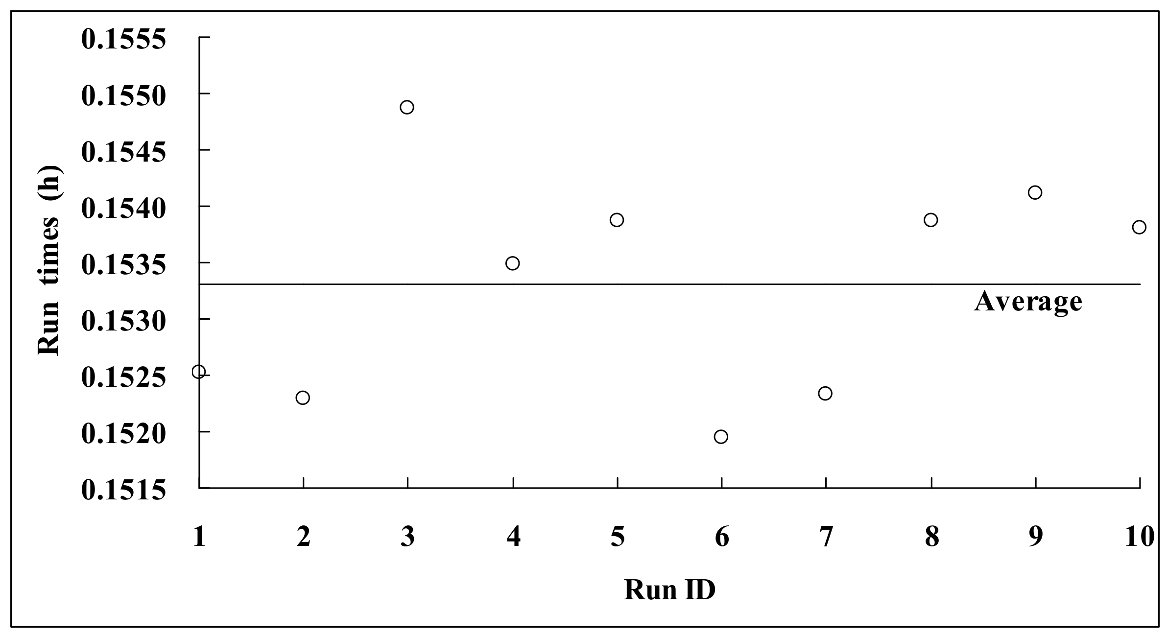
To analyze the stability of run time for replicate running, we have implemented the multiple replicate runs, up to 10 times, by using the Mesh-1 and the GPU computing. Figure 12 shows the run time distribution, from which it can be seen that the standard deviation is 3.3 s, which is on the order of seconds. Since the average run time is about 0.15 h, and the standard deviation is far below the average run time, it can be concluded that the run time of one running can be used for performance analysis.

For the three mesh division schemes of the flood control protection zone of the Wei River right bank, the different capacity levels were compiled on both the CPU and the GPU device.

Table 2. The test case of real flood simulation in the Wei River: results of different calculation schemes (T = running time; S = speedup ratio; TS = time saving ratio).

Mesh Type	Grid Number	Average Grid Area (m2)	TCPU (h)	TGPU (h)	S	TS (%)
Mesh-1	179,296	53,000	1.70	0.15	11.3	91
Mesh-2	717,184	13,250	10.69	0.62	17.2	94
Mesh-3	2,868,736	3313	86.72	2.79	31.1	97

gives the running time, speedup ratio, and time-saving ratio of the calculations, from which it can be seen that all three cases attained a dramatic reduction in running time. For mesh-1 of 179,296 grids, the 878 h (36.6 days) flood inundation process took approximately 1.70 h to calculate with the serial model, whereas only 0.15 h was required with a parallel model on the GPU K20 card (Nvidia, CA, USA). For mesh-2 of 717,184 grids, the 878 h (36.6 days) flood inundation process required approximately 10.69 h to calculate with a serial model. With the GPU-based parallel model, only 0.62 h were needed to complete the flood simulation. Furthermore, for mesh-3 of 2,868,736 grids, the running time of the serial model and parallel model are 86.72 h and 2.79 h, respectively. Since the accuracy of the flood simulation is largely dependent upon the topographical resolution, it can be concluded that the precision and speed of the flood model can be improved by mesh refinement and parallel computing, and the proposed GPU-based parallel model will contribute to large-scale flood simulations and real-time responses of disaster prevention and mitigation.

The running time, speedup ratio, and time-saving ratio all increased with the number of grids. Additionally, the speedup ratio and time-saving ratio also improved as the number of grids increased. For the three mesh division schemes, the speedup ratios of 11.3, 17.2, and 31.1 were achieved with 179,296, 717,184, and 2,868,736 grids, respectively. Thus, it can be concluded that the parallel model performs better with an increased grid number. In the view of real-time simulation, the calculation scheme using mesh-2 would be the best for the tradeoff between computational speed and mesh resolution.

5. Conclusions

A two-dimensional shallow water model was established for flood simulation based on an unstructured Godunov-type finite volume scheme. The MUSCL-Hancock scheme was used for time-stepping, and the HLLC approximate Riemann solver was used for computation of the fluxes. The main computational subroutines were presented as loops with data independence and natural parallelism. Thus, in a computational time-step, the calculations for each cell or edge are numerically decoupled, and the computational loops can be executed in parallel.

To realize a fast simulation of large-scale floods on a personal computer, a GPU-based high-performance computing method using the OpenACC application was adopted to parallelize the shallow water model. An unstructured data management method was presented to control the data transportation between the GPU and CPU with minimal overhead, and then both computation and data were offloaded from the CPU to the GPU, which can exploit the computational capability of the GPU as much as possible. As the finite volume scheme adopted in this work is explicit, and there is no correlation between grid calculations in a computational step, OpenACC clauses can be directly added to the original serial model codes to realize GPU computation, accelerating the program in an incrementally developing way with minimal recoding work.

The parallel model was validated through two benchmark cases. Furthermore, the flood control protection zone of the Wei River right bank was used as a case study. The total area is about 9503 km², and three grid division schemes with different resolutions were considered to test the performance of the parallel model, which was executed on the NVIDIA Kepler K20 platform (Nvidia, CA, USA). Results show that all three cases attained a dramatic reduction in the running time by using the GPU-based parallel model. For the mesh-1 of 179,296 grids, the 878 h (36.6 days) flood inundation process took approximately 1.70 h to calculate with the serial model, whereas only 0.15 h was required with a parallel model on the GPU K20 card. For the mesh-3 of 2,868,736 grids, the running times of the serial model and parallel model are 86.72 h and 2.79 h, respectively. Additionally, the running time, speedup ratio, and time-saving ratio all increased with the number of grids. For the three mesh division schemes, the speedup ratios of 11.3, 17.2, and 31.1 were achieved with 179,296, 717,184, and 2,868,736 grids, respectively. Since the accuracy of flood simulations is largely dependent upon the topographical resolution, it can be concluded that the precision and speed of the flood model can be improved by mesh refinement and parallel computing, and the proposed GPU-based parallel model will contribute to large-scale flood simulations and the real-time response of disaster prevention and mitigation.

References

- Song, L.; Zhou, J.; Guo, J.; Zou, Q.; Liu, Y. A robust well-balanced finite volume model for shallow water flows with wetting and drying over irregular terrain. Adv. Water Resour. 2011, 34, 915–932. [Google Scholar] [CrossRef]
- Bi, S.; Zhou, J.; Liu, Y.; Song, L. A finite volume method for modeling shallow flows with Wet-Dry fronts on adaptive cartesian grids. Math. Probl. Eng. 2014, 2014, 805–808. [Google Scholar] [CrossRef]
- Wu, G.; He, Z.; Liu, G. Development of a cell-centered godunov-type finite volume model for shallow water flow based on unstructured mesh. Math. Probl. Eng. 2014, 2014, 1–15. [Google Scholar] [CrossRef]
- Liu, Q.; Qin, Y.; Zhang, Y.; Li, Z. A coupled 1D–2D hydrodynamic model for flood simulation in flood detention basin. Nat. Hazards 2015, 75, 1303–1325. [Google Scholar] [CrossRef]
- Rehman, K.; Cho, Y.S. Novel slope source term treatment for preservation of quiescent steady states in shallow water flows. Water 2016, 8, 488. [Google Scholar] [CrossRef]
- Kvočka, D.; Ahmadian, R.; Falconer, R.A. Flood inundation modelling of flash floods in steep river basins and catchments. Water 2017, 9, 705. [Google Scholar] [CrossRef]
- Chen, J.; Zhong, P.-A.; Wang, M.-L.; Zhu, F.-L.; Wan, X.-Y.; Zhang, Y. A risk-based model for real-time flood control operation of a cascade reservoir system under emergency conditions. Water 2018, 10, 167. [Google Scholar] [CrossRef]
- Sanders, B.F.; Schubert, J.E.; Detwiler, R.L. ParBreZo: A parallel, unstructured grid, Godunov-type, shallow-water code for high-resolution flood inundation modeling at the regional scale. Adv. Water Resour. 2010, 33, 1456–1467. [Google Scholar] [CrossRef]
- Lai, W.; Khan, A.A. A parallel two-dimensional discontinuous galerkin method for shallow-water flows using high-resolution unstructured meshes. J. Comput. Civ. Eng. 2016, 31, 04016073. [Google Scholar] [CrossRef]
- Wang, X.; Shangguan, Y.; Onodera, N.; Kobayashi, H.; Aoki, T. Direct numerical simulation and large eddy simulation on a turbulent wall-bounded flow using lattice boltzmann method and multiple GPUs. Math. Probl. Eng. 2014, 2014, 1–10. [Google Scholar] [CrossRef]
- Wang, Y.; Yang, X. Sensitivity analysis of the surface runoff coefficient of HiPIMS in simulating flood processes in a Large Basin. Water 2018, 10, 253. [Google Scholar] [CrossRef]
- Zhang, S.; Yuan, R.; Wu, Y.; Yi, Y. Parallel computation of a dam-break flow model using OpenACC applications. J. Hydraul. Eng. 2016, 143, 04016070. [Google Scholar] [CrossRef]
- Zhang, S.; Li, W.; Jing, Z.; Yi, Y.; Zhao, Y. Comparison of three different parallel computation methods for a two-dimensional dam-break model. Math. Probl. Eng. 2017, 2017, 1–12. [Google Scholar] [CrossRef]
- Liang, Q.; Xia, X.; Hou, J. Catchment-scale high-resolution flash flood simulation using the GPU-based technology. Procedia Eng. 2016, 154, 975–981. [Google Scholar] [CrossRef]
- Zhao, X.D.; Liang, S.X.; Sun, Z.C.; Zhao, X.Z.; Sun, J.W.; Liu, Z.B. A GPU accelerated finite volume coastal ocean model. J. Hydrodyn. 2017, 29, 679–690. [Google Scholar] [CrossRef]
- Chen, T.Q.; Zhang, Q.H. GPU acceleration of a nonhydrostatic model for the internal solitary waves simulation. J. Hydrodyn. 2013, 25, 362–369. [Google Scholar] [CrossRef]
- Wu, J.; Zhang, H.; Yang, R.; Dalrymple, R.A.; Hérault, A. Numerical modeling of dam-break flood through intricate city layouts including underground spaces using GPU-based SPH method. J. Hydrodyn. 2013, 25, 818–828. [Google Scholar] [CrossRef]
- Néelz, S.; Pender, G. Benchmarking the Latest Generation of 2D Hydraulic Modelling Packages; Environment Agency: Bristol, UK, 2013. [Google Scholar]
- Ying, X.; Khan, A.A.; Wang, S.S.Y. Upwind conservative scheme for the Saint Venant equations. J. Hydraul. Eng. 2004, 130, 977–987. [Google Scholar] [CrossRef]
Figure 1.
The computational flow diagram for a GPU-based parallel model.
Figure 2.
Plan and profile of the DEM used in the test case of flooding a disconnected water body [18].
Figure 3.
The computed water levels at points P1 and P2 in the test case of flooding a disconnected water body: (a) computed results of the present model at P1 and P2; (b) computed results of different models at P1; (c) computed results of different models at P2.
Figure 4.
The plan view of the topography of the Toce River physical model.
Figure 5.
The inflow discharge boundary condition of the Toce River physical model.
Figure 6.
Comparison of the stage-time hydrographs in the Toce River physical model.
Figure 7.
The flood control protection zone of the Wei River right bank (the blocks of hatch pattern with blue, yellow, and green belong to Henan Province, Hebei Province, and Shandong Province, respectively).
Figure 8.
The topography of the flood control protection zone of the Wei River right bank.
Figure 9.
The test case of real flood simulation in the Wei River: the discharge across the hypothetical dyke breach (the dyke breach occurred at time t = 0).
Figure 10.
The test case of real flood simulation in the Wei River: the distribution of the computed water depth at different times using Mesh-1.
Figure 11.
The test case of real flood simulation in the Wei River: the water volume of inflow and the cells’ storage.
Figure 12.
The test case of real flood simulation in the Wei River: the run time distribution of replicate running by using the Mesh-1 and the GPU computing.