Brooks–Corey Modeling by One-Dimensional Vertical Infiltration Method

Abstract

The laboratory methods used for the soil water retention curve (SWRC) construction and parameter estimation is time-consuming. A vertical infiltration method was proposed to estimate parameters α and n and to further construct the SWRC. In the present study, the relationships describing the cumulative infiltration and infiltration rate with the depth of the wetting front were established, and simplified expressions for estimating α and n parameters were proposed. The one-dimensional vertical infiltration experiments of four soils were conducted to verify if the proposed method would accurately estimate α and n. The fitted values of α and n, obtained from the RETC software, were consistent with the calculated values obtained from the infiltration method. The comparison between the measured SWRCs obtained from the centrifuge method and the calculated SWRCs that were based on the infiltration method displayed small values of root mean square error (RMSE), mean absolute percentage error (MAPE), and mean absolute error. SWMS_2D-based simulations of cumulative infiltration, based on the calculated α and n, remained consistent with the measured values due to small RMSE and MAPE values. The experiments verified the proposed one-dimensional vertical infiltration method, which has applications in field hydraulic parameter estimation.

1. Introduction

The soil water retention curve (SWRC) represents the soil’s ability to store and release water as it is subjected to soil suction, and is described as the relation between soil moisture and soil suction [1,2]. The SWRC is used to evaluate the size and the distribution of soil pores and its water-holding capacity [3,4]. Soil hydraulic parameters can be obtained from the SWRC and used as key inputs for the water movement prediction that simulates the evaporation, the infiltration, and the runoff dynamics of field soils. Further, these parameters can be used to estimate the functions of various hydraulic properties of unsaturated and saturated soils to model solute transport [5,6]. The soil water retention behavior is important for many applications.

The soil hydraulic parameters primarily include θ_s, θ_r, α, and n, which can be estimated from the SWRC [7]. Numerous techniques are employed for the SWRC determination, such as the pressure plate method, the filter paper method, the tensiometer method, the osmotic suction control method, and the centrifuge method. Xing et al. [8] indicated that soil samples exhibit compressibility under a centrifugal force when using the centrifuge method—which can lead to clear changes in the bulk density—and similar problems are found with the tensiometer technique and the pressure plate technique [9,10,11]. The collected soil moisture data for the SWRC requires correction. Previous research [12] called for these corrections because accurate data collection during SWRC measurement enhances the accuracy of the obtained hydraulic parameters. These methods are time-consuming, requiring a measurement of the sedimentation of soil samples, whereas the change in bulk density is easily ignored [6,13,14]. Due to the shortcomings of SWRC data collection, direct SWRC measurements were avoided in this study. The key parameters α and n were estimated through one-dimensional vertical infiltration experiments, followed by SWRC construction. The adopted method (i.e., the field-infiltration method) matched the actual field situation, where water infiltration is common. In order to simplify field operation, we used simplified visual observation and calculation for parameter estimation. The relationships describing the cumulative infiltration and the infiltration rate with the depth of wetting front are presented.

The main purposes of this study were to verify if the selected method was effective for parameter estimation during SWRC construction and to verify if the obtained SWRC was effective for the cumulative infiltration prediction. Specifically, the aims were (1) to provide a simplified and practical method to estimate soil hydraulic parameters and SWRCs and (2) to investigate the effect that the estimated SWRC obtained through the one-dimensional vertical infiltration method had on cumulative infiltration simulations when using SWMS_2D (Version 1.21, U.S. Department of Agriculture, Riverside, CA, USA), a Fortran-based open-source software package, which is simpler than HYDRUS for modeling soil water dynamics [8,15].

2. Theory

The one-dimensional infiltration process can be described by Equation (1). The initial and boundary conditions are shown in Equations (2) and (3), respectively.

$$\frac{\partial \theta }{\partial t}=\frac{\partial }{\partial z}\left(D\left(\theta \right)\frac{\partial \theta }{\partial z}\right)-\frac{\partial K\left(\theta \right)}{\partial z}$$

(1)

$$\theta ={\theta }_{0}0\le z\le H_{\mathrm{z}},t=0$$

(2)

$$\{\begin{array}{l}\theta ={\theta }_{\mathrm{s}}z=0,t>0\\ \theta ={\theta }_{0}z=H_{\mathrm{z}},t>0\end{array}$$

(3)

where D represents unsaturated soil water diffusivity (cm²/min), K represents unsaturated hydraulic conductivity (cm/min), z represents the depth from the soil surface (cm, taken positive downward), H_z represents the depth of simulation domain (cm), and t represents time (min).

Parlange [16] stated that the value of ${\displaystyle {\int }_{\theta }^{{\theta }_{\mathrm{s}}}\frac{\partial z}{\partial t}\mathrm{d}\theta }$ in the integral equation of Equation (1) was approximately 0 under a small z condition. The integral equation of Equation (1) was simplified:

$$-D\left(\theta \right)\frac{\partial \theta }{\partial z}+K\left(\theta \right)=-D\left({\theta }_{\mathrm{s}}\right)\frac{\partial {\theta }_{\mathrm{s}}}{\partial z}+K\left({\theta }_{\mathrm{s}}\right)$$

(4)

The infiltration rate i at any time equals the water flux at the soil surface (Equation (5)):

$$i={\left(-D\left(\theta \right)\frac{\partial \theta }{\partial z}+K\left(\theta \right)\right)}_{z=0}$$

(5)

Equation (5) is described as Equation (6) in the form of soil suction, with combinations of $K\left(\theta \right)=C\left(\theta \right)D\left(\theta \right)$ and $C\left(\theta \right)=-\mathrm{d}\theta /\mathrm{d}h$.

$$i=K\frac{\mathrm{d}h}{\mathrm{d}z}+K$$

(6)

The unsaturated hydraulic conductivity was calculated as Equation (7) [17]:

$$K\left(h\right)=K_{\mathrm{s}}{e}^{-\alpha h}$$

(7)

The differentiation of Equation (7) was substituted into Equation (6), and the obtained equation (i.e., $-\alpha {\displaystyle {\int }_0^z\mathrm{d}}z={\displaystyle {\int }_{K_{\mathrm{s}}}^K\frac{\mathrm{d}K}{i-K}}$) was integrated into Equation (8).

$$-\alpha z=\ln \frac{i-K_{\mathrm{s}}}{i-K}$$

(8)

From Equation (8), the K corresponding to any depth z could be obtained Equation (9). When z equaled the depth of the wetting front (i.e., z = z_f), θ denoted the initial soil moisture. K could be ignored under a low soil moisture condition. Under this circumstance, Equation (8) was simplified into Equation (10).

$$K=i-\left(i-K_{\mathrm{s}}\right)e^{\alpha z}$$

(9)

$$i=\frac{K_{\mathrm{s}}}{1-e^{-\alpha z_f}}$$

(10)

Taylor series expansions (first order) of Equations (9) and (10) were approximately obtained, displayed as Equations (11) and (12):

$$K=K_{\mathrm{s}}-\alpha z\left(i-K_{\mathrm{s}}\right)$$

(11)

$$i=\frac{K_{\mathrm{s}}}{\alpha z_f}+K_{\mathrm{s}}$$

(12)

In addition, the expression of the soil water retention curve (SWRC) was described via Equation (13), based on Brooks–Corey model [18].

$$\frac{\theta -{\theta }_{\mathrm{r}}}{{\theta }_{\mathrm{s}}-{\theta }_{\mathrm{r}}}={\left(\alpha h\right)}^{-n}$$

(13)

where θ_r and θ_s represents the residual and saturated soil moisture, respectively, (cm³/cm³), h represents the soil suction (cm), α represents the inverse of the air-entry value (1/cm), and n represents the curve-fitting parameter.

Equations (7), (11), and (12) were combined (i.e., $\alpha h=-\ln \frac{K}{K_{\mathrm{s}}}$ and $\frac{K}{K_{\mathrm{s}}}=1-\frac{z}{z_f}$) so that Equation (13) could be rewritten as Equation (14).

$$\frac{\theta -{\theta }_{\mathrm{r}}}{{\theta }_{\mathrm{s}}-{\theta }_{\mathrm{r}}}={\left[-\ln \left(1-\frac{z}{z_f}\right)\right]}^{-n}$$

(14)

The cumulative infiltration corresponding to z_f is expressed as:

$$I={\displaystyle {\int }_0^{z_f}\left(\theta -{\theta }_0\right)\mathrm{d}z}$$

(15)

where I represents the cumulative infiltration (cm) and θ₀ represents the initial soil moisture (cm³/cm³).

The Taylor series expansion (first order) of Equation (14) was approximately obtained, displayed as Equation (16). Equation (16) was substituted into the Equation (15) in order to obtain Equation (17).

$$\theta ={\theta }_{\mathrm{r}}+\left({\theta }_{\mathrm{s}}-{\theta }_{\mathrm{r}}\right){\left(\frac{z}{z_f}\right)}^{-n}$$

(16)

$$I=\left[\frac{1}{1-n}\left({\theta }_{\mathrm{s}}-{\theta }_{\mathrm{r}}\right)+\left({\theta }_{\mathrm{r}}-{\theta }_0\right)\right]z_f$$

(17)

Linear relationships between i and 1/z_f and I and z_f were taken from Equations (18) and (19).

$$i=\frac{A_1}{z_f}+A_2;A_1=\frac{K_{\mathrm{s}}}{\alpha },A_2=K_{\mathrm{s}}$$

(18)

$$I=A_3{z}_f;A_3=\frac{1}{1-n}\left({\theta }_{\mathrm{s}}-{\theta }_{\mathrm{r}}\right)+\left({\theta }_{\mathrm{r}}-{\theta }_0\right)$$

(19)

The parameters α and n were estimated through the following Equation:

$$\{\begin{array}{l}\alpha =A_2/A_1\\ n=1-\frac{{\theta }_{\mathrm{s}}-{\theta }_{\mathrm{r}}}{A_3-\left({\theta }_{\mathrm{r}}-{\theta }_0\right)}\end{array}$$

(20)

3. Materials and Methods

3.1. Soil Sample Collection and SWRC Measurement

Loam and sandy loam (

Table 1. Particle size distribution of the experimental soils.

Soil Type	Particle Size Distribution/%			θs/(cm3/cm3) e	θr/(cm3/cm3) f	Designed γd/(g/cm3) g	SOC/(g/kg) h
	0–0.002 mm	0.002–0.02 mm	0.02–2 mm
Sandy loam a	9.24	22.01	68.75	0.502	0.04	1.10~1.13	16.50
Sandy loam b	15.59	20.53	63.88	0.327	0.03	1.51~1.55	4.52
Loam c	17.12	38.65	44.23	0.363	<0.001	1.51~1.56	2.23
Loam d	19.00	34.94	46.06	0.481	0.06	1.30~1.33	6.65

Note: ^a Soils collected from Liaoning Province; ^b soils collected from Xinjiang Province; ^c soils collected from Shandong Province; ^d soils collected from Shaanxi Province; ^e θ_s represents the saturated soil moisture; ^f θ_r represents the residual soil moisture; ^g γ_d represents the initial dry bulk density; ^h SOC represents the soil organic carbon.

) were selected from the cultivated field soil layers in Liaoning, Shandong, Shaanxi, and Xinjiang Provinces in China. Liaoning Province is located on the northeast plain, where cultivated farmland soil is primarily nutrient-rich black soil. Shandong Province has extensive river systems, which feed into the Bohai Sea and the Yellow Sea, resulting in moist and brown soils. Shaanxi Province is located on the Loess Plateau, which is full of loose soils. Xinjiang region has strong atmospheric evaporation and little rainfall, creating a saline–alkali soil. Soil samples were selected to represent their respective regions.

A moderate amount of scattered soil from each sample was compacted into cutting rings (100 cm³) at the designated bulk density (Table 1), and then saturated with distilled water for 48 h. The soil samples were placed into a centrifuge (CR21G II, HITACHI, Tokyo, Japan) to obtain SWRC data for the four soils. In order to avoid compressibility during centrifugation, some low suctions were set, including 100 cm, 200 cm, 300 cm, 400 cm, 500 cm, 600 cm, 700 cm, 800 cm, and 1000 cm. After the equilibrium time for a particular suction was obtained, the soil samples were then removed from the centrifuge and weighed on an electronic balance with a precision of 0.01 g. The soil samples were oven dried at 105 °C until a constant weight was obtained. The SWRCs for the four experimental soils were constructed in accordance with the θ–h parameter planes.

3.2. Laboratory One-Dimensional Infiltration

The soils were compacted into the Plexiglas columns at the designated dry bulk density in order to simulate the in situ bulk density of a local cultivated field, with an initial soil moisture of approximately 0.25 cm³/cm³. The depth of soil compaction was 20 cm. The soils were compacted into soil columns and left for 24 h until the infiltration experiment was conducted. Each treatment was performed thrice. A graduated Marriott bottle filled with distilled water was connected to the top of each soil column to maintain a steady infiltration head at 5 cm, as well as a continuous water supply. The water level in the Marriott bottle and the depth of wetting front were recorded. The time interval was 1, 2, 3, and 5 min during the processes of durations 1~10, 10~30, 30~60, and >60 min, respectively. The infiltration finished when the wetting front reached a depth of 20 cm. The cumulative infiltration and the depth of the wetting front were used to estimate the α and n parameters and for further constructing the SWRC.

3.3. Error Analysis

Root mean square error (RMSE), the mean absolute percentage error (MAPE), and the mean absolute error (MAE)—Equations (21)–(23), respectively—were selected to conduct a differential analysis between the measured and the calculated soil moisture. The first two indicators evaluated the differences between the measured cumulative infiltration and the calculated measurement using the parameters obtained via the infiltration method. A small value of RMSE, MAPE, or MAE indicated a high predictive accuracy [19].

$$RMSE=\sqrt{\frac{1}{p}\cdot {\displaystyle \sum _{i=1}^p{\left(V_i-{\widehat{V}}_i\right)}^2}}$$

(21)

$$MAPE=\frac{1}{p}{\displaystyle \sum _{i=1}^p\left|\frac{V_i-{\widehat{V}}_i}{V_i}\right|}\times 100\%$$

(22)

$$MAE=\frac{1}{p}{\displaystyle \sum _{i=1}^p\left|V_i-{\widehat{V}}_i\right|}$$

(23)

where p is the sample size, $V_i$ is the ith measured soil moisture or cumulative infiltration, and ${\widehat{V}}_i$ is the ith calculated soil moisture or the cumulative infiltration.

4. Results

4.1. Comparison of the Fitted and Calculated Values of α and n

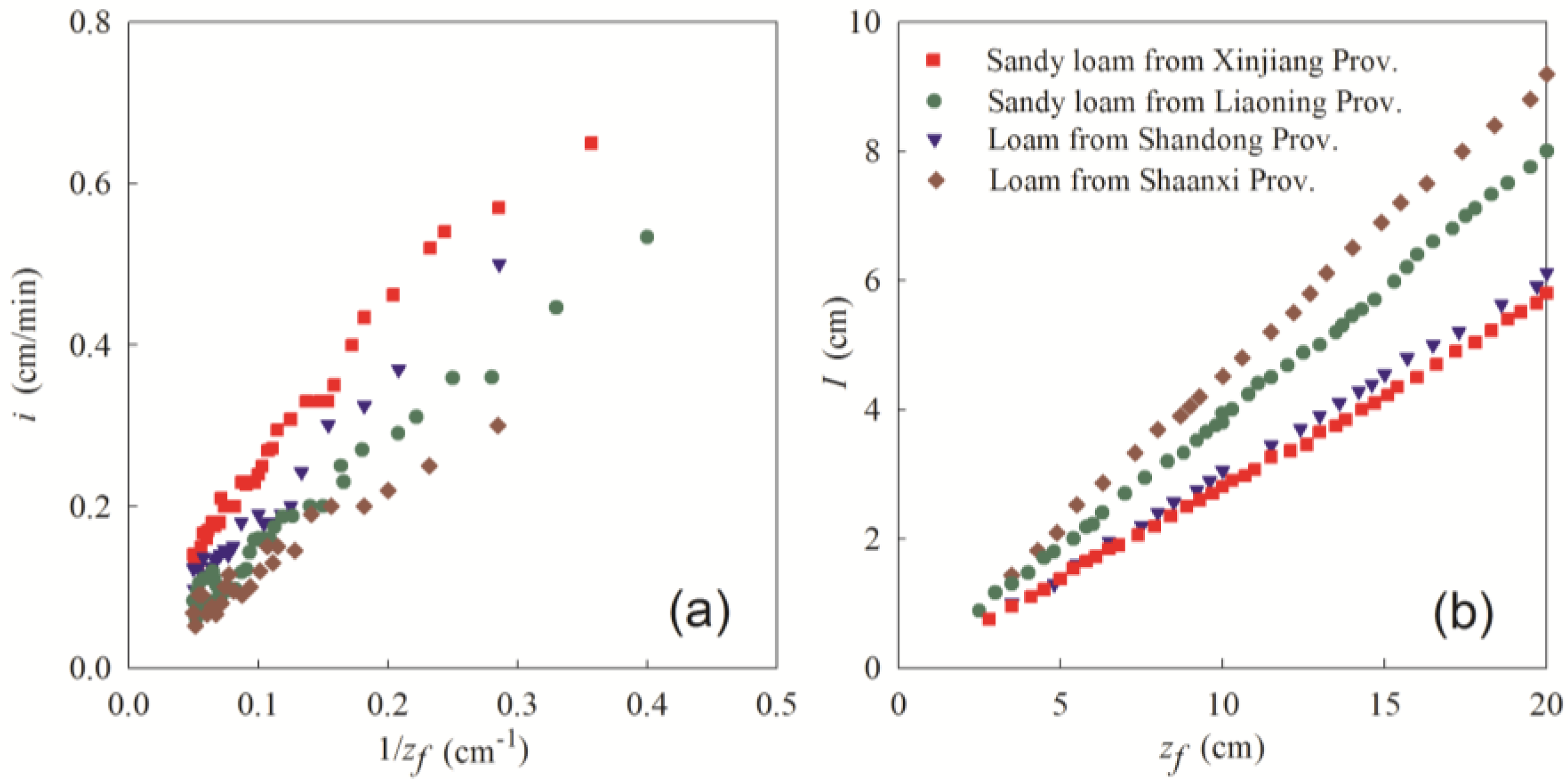
The measured data from the thrice-replicated samples of all four soils demonstrated a similar tendency between i and 1/z_f and I and z_f, showing that i and I increased as 1/z_f and z_f increased. The mean values were used to construct Figure 1 to highlight the relationships. Equations (18) and (19) revealed that the non-zero-axial and zero-axial linear functions were used to fit i–1/z_f and I–z_f curves. The values of parameters A₁, A₂, and A₃ (listed in

Table 2. Parameter values for equations i and 1/z_f and I and z_f.

Experimental Soils	A1	A2	R2	A3	R2
Sandy loam from Liaoning Province	1.2811	0.0238	0.9712	0.3969	0.9845
	1.2025	0.0221	0.9697	0.3711	0.9912
	1.2404	0.0232	0.9812	0.3870	0.9953
	1.2413	0.0230	0.9689	0.3850	0.9980
Sandy loam from Xinjiang Province	1.8720	0.0345	0.9845	0.3108	0.9976
	1.8558	0.0310	0.9674	0.2814	0.9918
	1.8403	0.0306	0.9621	0.2764	0.9920
	1.8560	0.0320	0.9775	0.2895	0.9987
Loam from Shandong Province	1.5521	0.0238	0.9810	0.2974	0.9950
	1.5546	0.0248	0.9755	0.3001	0.9899
	1.5389	0.0234	0.9733	0.2990	0.9978
	1.5485	0.0240	0.9793	0.2988	0.9988
Loam from Shaanxi Province	0.8740	0.0199	0.9589	0.4101	0.9984
	0.8785	0.0211	0.9746	0.4181	0.9973
	0.8939	0.0221	0.9810	0.4349	0.9892
	0.8821	0.0210	0.9633	0.4210	0.9972

Note: The bolded font represents the mean value of all replicates, all other data are the value for each replicate.

) displayed a good linear relationship between i and 1/z_f and I and z_f due to a high R² (>0.95). The results justified Equations (18) and (19).

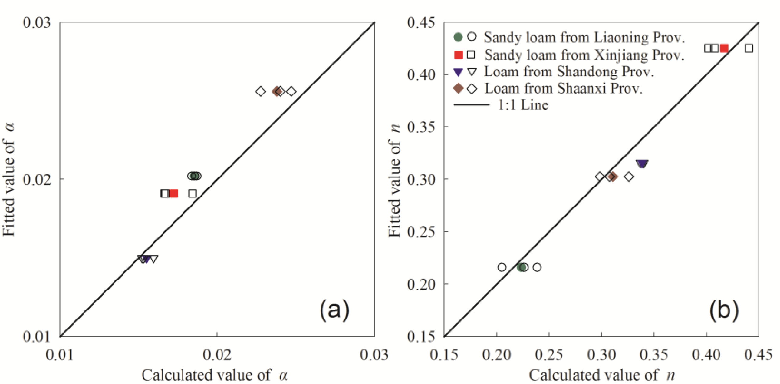
The parameter α and n values were calculated using Equation (20). The fitted values were obtained from the RETC software (Agricultural Research Service, Riverside, CA, USA) using the measured data from the centrifuge method. Figure 2 shows that the α and n datasets were around the 1:1 line. The mean values of the relative error between the fitted and the calculated α were 8.27%, 9.73%, 3.33%, and 7.00% for the soil from Liaoning, Xinjiang, Shandong, and Shaanxi. The values for samples between the fitted and the calculated n were 3.49%, 1.91%, 7.21%, and 2.80%.

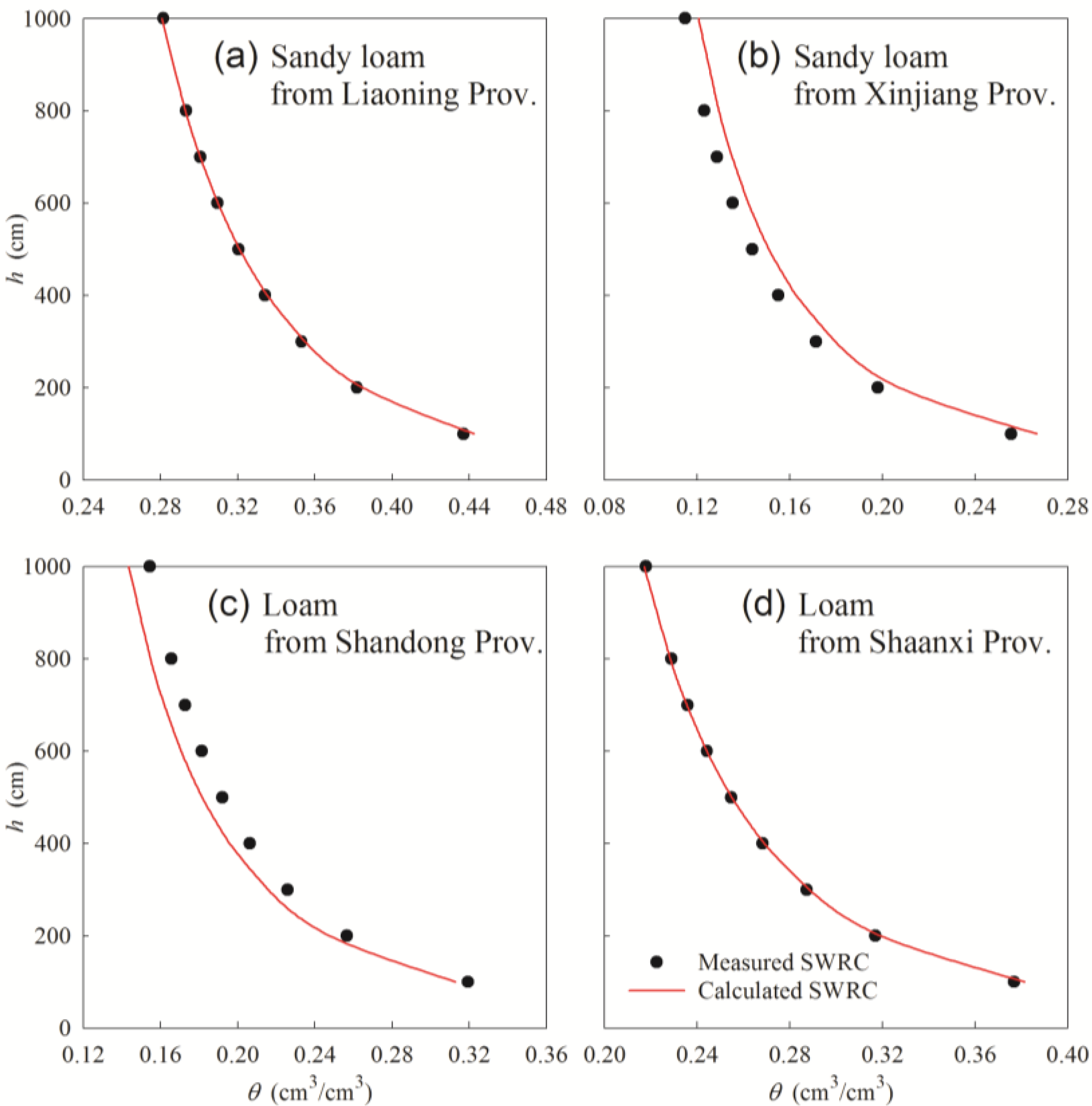
4.2. Comparison of the Measured and Calculated SWRCs

The SWRC generated via the measured θ–h data planes, obtained from centrifuge method, was defined as the measured SWRC. The generated SWRC, combined with the α and n obtained from the infiltration method, was defined as the calculated SWRC. The measured and calculated SWRCs for the four soils (plotted in Figure 3) demonstrated a good identity of the two types of the SWRC. The measured soil moisture for each tested suction was similar to the fitted soil moisture. Further error analysis showed that the correlation coefficient r between the measured and the calculated soil moisture for all four soils were larger than 0.99. The RMSE and MAE values were slightly larger than 0, demonstrating a near perfect estimation result. This result was also due to small MAPE values (

Table 3. Error analysis for the measured and calculated soil moisture contents.

Experimental Soils	RMSE/(cm3/cm3)	MAE/(cm3/cm3)	MAPE/%
Sandy loam from Liaoning Province	0.0023	0.0015	0.3989
Sandy loam from Xinjiang Province	0.0078	0.0076	4.8849
Loam from Shandong Province	0.0101	0.0100	5.1445
Loam from Shaanxi Province	0.0018	0.0012	0.3806

). The observed SWRCs of the experimental soils and the error values indicated that using the one-dimensional vertical infiltration method for parameter estimation (i.e., α and n) and for the SWRC estimation was reasonable.

4.3. Performance of Cumulative Infiltration Simulation

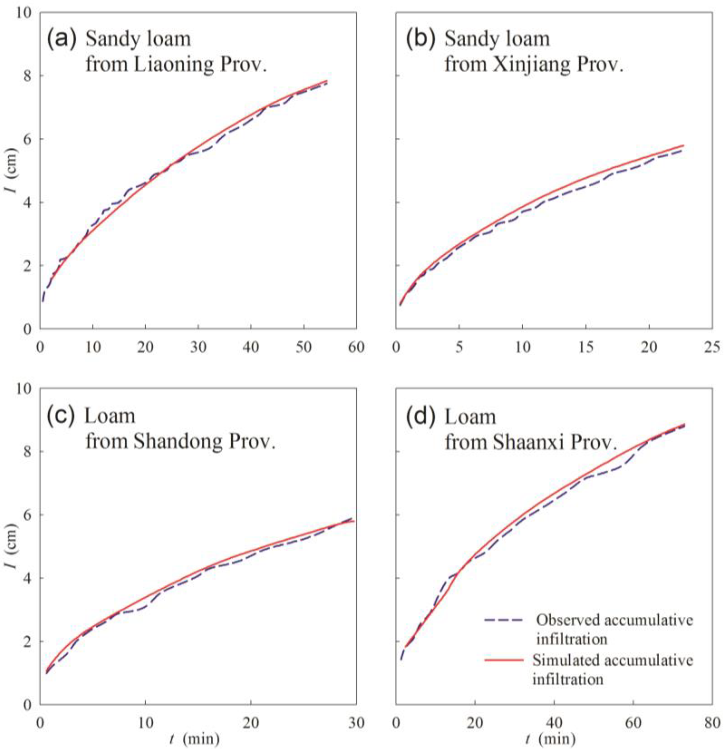
The cumulative infiltration was simulated via SWMS_2D software, using the α and n parameters obtained by the infiltration method. The changes of simulated cumulative infiltration over time remained consistent with the observed values, although some gaps were exposed (Figure 4). The errors demonstrated that the RMSE and MAPE values between the observed and simulated values were 0.0698 cm and 2.0234% for the sandy loam from Liaoning, 0.1453 cm and 4.3688% for the sandy loam from Xinjiang, 0.1139 cm and 3.5108% for the loam from Shandong, and 0.1529 cm and 2.7700% for the loam from Shaanxi. The small RMSE and MAPE values indicated that the infiltration method had potential for parameter estimation (i.e., α and n), which could be considered as the inputs for the SWMS_2D.

5. Summary and Conclusions

In the present study, three sets of α and n values were calculated through a one-dimensional infiltration experiment (Figure 2). The standard deviations of α were 1.34 × 10⁻⁴, 8.32 × 10⁻⁴, 3.26 × 10⁻⁴, and 8.08 × 10⁻⁴, and n reached 0.0139, 0.0170, 0.0013, and 0.0116 for the soil from Liaoning, Xinjiang, Shandong, and Shaanxi, respectively. The small standard deviations indicated the calculated α and n values were accurate via the infiltration method, although additional soils and duplicate tests remain necessary. Ma et al. [20] and Wang et al. [21] proposed a horizontal infiltration method to estimate the parameters of the Brooks–Corey model. The present study adopted the vertical infiltration method for parameter estimation, which would be more practical since water infiltration is a more common in the cropland, particularly after irrigation events. In these studies, undisturbed 20 cm depth soil samples were obtained for the hydraulic parameters that were estimated through the vertical infiltration method, which would save more time than the direct SWRC measurements. Su et al. [22] used second-, third-, and fourth-order Taylor series expansions to obtain an approximate analytical solution for a one-dimensional, constant water head, vertical infiltration. This study, however, used first-order Taylor series expansion for parameter estimation with satisfying accuracy, which simplified the calculation. The SWRCs were ultimately determined based on the calculated α and n, which were considered the inputs for the accumulation infiltration simulation. This justified the obtained SWRCs via the one-dimensional vertical infiltration method.

The theoretical relationships between I and i and z_f were established, and a simplified parameter for estimating expressions of α and n was proposed. One-dimensional vertical infiltration experiments of the four loam and sandy loam soils showed linear relationships between i and 1/z_f and I and z_f. The calculated values of α and n obtained through the infiltration method were consistent with the fitted values obtained from the RETC software (Agricultural Research Service, Riverside, CA, USA), with a relative error of 3.33–9.73% and 1.91–7.21%. The values of soil moisture for the calculated SWRCs were similar to the measured SWRCs, with a RMSE of 0.0018–0.0101 cm³/cm⁻³, a MAE of 0.0012–0.0100 cm³/cm⁻³, and a MAPE of 0.3806–5.1445%. The SWMS_2D-based cumulative infiltration simulations for the four soils revealed that the simulated values (on the basis of calculated α and n) were consistent with the observed values, demonstrated by the small RMSE (0.0698–0.1529 cm) and MAPE (2.0234–4.3688%).

References

- Gao, Y.; Sun, D. Soil-water retention behavior of compacted soil with different densities over a wide suction range and its prediction. Comput. Geotech. 2017, 91, 17–26. [Google Scholar] [CrossRef]
- Pham, H.Q.; Fredlund, D.G. Equations for the entire soil-water characteristic curve of a volume change soil. Can. Geotech. J. 2008, 45, 443–453. [Google Scholar] [CrossRef]
- Wong, J.T.F.; Chen, Z.; Chen, X.; Ng, C.W.W.; Wong, M.H. Soil-water retention behavior of compacted biochar-amended clay: A novel landfill final cover material. J. Soil Sediments 2017, 17, 590–598. [Google Scholar] [CrossRef]
- Xing, X.; Kang, D.; Ma, X. Differences in loam water retention and shrinkage behavior: Effects of various types and concentrations of salt ions. Soil Tillage Res. 2017, 167, 61–72. [Google Scholar] [CrossRef]
- Ciocca, F.; Lunati, I.; Parlange, M.B. Effects of the water retention curve on evaporation from arid soils. Geophys. Res. Lett. 2014, 41, 3110–3116. [Google Scholar] [CrossRef]
- Zhou, W.H.; Yuen, K.V.; Tan, F. Estimation of soil-water characteristic curve and relative permeability for granular soils with different initial dry densities. Eng. Geol. 2014, 179, 1–9. [Google Scholar] [CrossRef]
- Garg, N.K.; Gupta, M. Assessment of improved soil hydraulic parameters for soil water content simulation and irrigation scheduling. Irrig. Sci. 2015, 33, 247–264. [Google Scholar] [CrossRef]
- Xing, X.; Li, Y.; Ma, X. Water retention curve correction using changes in bulk density during data collection. Eng. Geol. 2018, 233, 231–237. [Google Scholar] [CrossRef]
- Boivin, P.; Garnier, P.; Vauclin, M. Modeling the soil shrinkage and water retention curves with the same equations. Soil Sci. Soc. Am. J. 2006, 70, 1082–1093. [Google Scholar] [CrossRef]
- Braudeau, E.; Sene, M.; Mohtar, R.H. Hydrostructural characteristic of two African tropical soils. Eur. J. Soil Sci. 2005, 56, 375–388. [Google Scholar] [CrossRef]
- Lu, D.; Shao, M.; Horton, R.; Liu, C. Effect of changing bulk density during water desorption measurement on soil hydraulic properties. Soil Sci. 2004, 169, 319–329. [Google Scholar] [CrossRef]
- Zhai, Q.; Rahardjo, H. Estimation of permeability function from the soil-water characteristic curve. Eng. Geol. 2015, 199, 148–156. [Google Scholar] [CrossRef]
- Fu, X.; Shao, M.; Lu, D.; Wang, H. Soil water characteristic curve measurement without bulk density changes and its implications in the estimation of soil hydraulic properties. Geoderma 2011, 167, 1–8. [Google Scholar] [CrossRef]
- Mohammadi, M.H.; Meskini-Vishkaee, F. Predicting soil moisture characteristic curves from continuous particle-size distribution data. Pedosphere 2013, 23, 70–80. [Google Scholar] [CrossRef]
- Yao, W.W.; Ma, X.Y.; Li, J.; Parkes, M. Simulation of point source wetting pattern of subsurface drip irrigation. Irrig. Sci. 2011, 29, 331–339. [Google Scholar] [CrossRef]
- Parlange, J.Y. Theory of water-movement in soils: I. One-dimensional absorption. Soil Sci. 1971, 111, 134–137. [Google Scholar] [CrossRef]
- Russo, D. Determining soil hydraulic properties by parameter estimation: On the selection of a model for the hydraulic properties. Water Resour. Res. 1988, 24, 453–459. [Google Scholar] [CrossRef]
- Brooks, R.H.; Corey, A.T. Hydraulic Properties of Porous Media; Hydraulic Papers; Colorado State University: Fort Collins, CO, USA, 1964. [Google Scholar]
- Xing, X.; Liu, Y.; Zhao, W.; Kang, D.; Yu, M.; Ma, X. Determination of dominant weather parameters on reference evapotranspiration by path analysis theory. Comput. Electron. Agric. 2016, 120, 10–16. [Google Scholar] [CrossRef]
- Ma, D.; Zhang, J.; Lai, J.; Wang, Q. An improved method for determining Brooks-Corey model parameters from horizontal absorption. Geoderma 2016, 263, 122–131. [Google Scholar] [CrossRef]
- Wang, Q.; Horton, R.; Shao, M. Horizontal infiltration method for determining Brooks-Corey model parameters. Soil Sci. Soc. Am. J. 2002, 66, 1733–1739. [Google Scholar] [CrossRef]
- Su, L.; Wang, J.; Qin, X.; Wang, Q. Approximate solution of a one-dimensional soil water infiltration equation based on the Brooks-Corey model. Geoderma 2017, 297, 28–37. [Google Scholar] [CrossRef]
Figure 1.
Relationships between i and 1/zf and between I and zf (the data are the mean values of the three replicates). (a) Relationship between i and 1/zf; (b) Relationship between I and zf.
Figure 2.
The fitted and calculated values the α and n parameters (hollow symbols represent the values of the three replicates, and the solid symbols represent the mean values of the three replicates). (a) Comparison of the fitted and calculated values of α; (b) Comparison of the fitted and calculated values of n.
Figure 3.
Measured and calculated soil water retention curves (SWRCs) for the experimental loam and sandy loam (the calculated SWRCs were obtained using the mean values of α and n from the three replicates). (a) The experimental soil is sandy loam collected from Liaoning Province; (b) The experimental soil is sandy loam collected from Xinjiang Province; (c) The experimental soil is loam collected from Shandong Province; (d) The experimental soil is loam collected from Shaanxi Province.
Figure 4.
Comparisons of the observed and simulated cumulative infiltration methods (the data for observed cumulative infiltration are the mean value of the three replicates). (a) The experimental soil is sandy loam collected from Liaoning Province; (b) The experimental soil is sandy loam collected from Xinjiang Province; (c) The experimental soil is loam collected from Shandong Province; (d) The experimental soil is loam collected from Shaanxi Province.