Performance Analysis of Ageing Single-Jet Water Meters for Measuring Residential Water Consumption


1
ITA—Grupo de Ingeniería y Tecnología del Agua, Dpto. de Ingeniería del Agua y Medio Ambiente, Universitat Politecnica Valencia, Camino de Vera s/n, 46022 Valencia, Spain
2
Smart Metering Manager, FACSA, Calle Mayor 82-84, 12001 Castellon, Spain
*
Author to whom correspondence should be addressed.
Water 2018, 10(5), 612; https://doi.org/10.3390/w10050612
Submission received: 23 March 2018
/
Revised: 18 April 2018
/
Accepted: 5 May 2018
/
Published: 8 May 2018
(This article belongs to the Special Issue Advances in the Economic Analysis of Residential Water Use)
Abstract
:Single-jet meters are one of the most frequently used domestic meters that can be found in water distribution systems. Like any other water meter technology, they have significant metrological limitations that prevent them, even if recently installed, from measuring all water consumption of a domestic customer. After installation, their metrological characteristics evolve depending on the particular design of the meters and their actual working conditions in the field. This work presents a comprehensive set of tests to determine the initial and after installation weighted error of two types of domestic single-jet water meters. Three non-linear degradation models have been derived from the tests results. These models consider age, totalised volume, or both parameters simultaneously as drivers of the weighted error. The results show that even though the construction of the two examined meters is similar, they have been working under comparable operational conditions and measuring water of the same quality, there is a significant difference in the performance between both types. This result highlights the need to conduct individual analyses for each meter type and the impossibility of generalizing conclusions on how the weighted error could evolve over time.
1. Introduction
Water losses have been identified as one of the leading problems common to any water utility in the world. High levels of losses can significantly affect future water resources availability, energy consumption associated to water production and distribution, overall quality of service to customers, water quality levels and operational costs and life of the assets. Depending on their nature, the International Water Association (IWA, London, UK) categorises water losses in two components [1]: real losses and apparent losses. Real losses are mainly caused by leakage in pipes, valves, tanks, and other elements in the network. Apparent losses include the volume of water stolen by the users, the measuring errors of the meters and data handling errors. While apparent losses volumes are typically smaller than real losses, these two components become almost equal when making the comparison in terms of revenue loss caused by the utility. This is because a cubic meter of water lost in a leak in the network has a cost to the utility equal to the production cost. On the contrary, a cubic meter supplied to a customer that is not measured by the water meter has a cost to the utility equal to the retail price of the last cubic meter of water sold to that customer. In addition, in a properly managed water supply system, apparent losses are mainly caused by water meter inaccuracies. Consequently, the water utility’s revenue strongly relies on the actual measuring performance of installed water meters.
While the published International Standards on water meters [2,3] mostly specify the metrological and technical requirements of new meters, there is a lack of international standards defining how the metrological performance of the meters should be after installation. Only very few countries have specific legislation or standards in relation to the metrological requirements of used meters. In addition to this, the number of parameters that can affect the actual accuracy of a water meter in the field is not small. Thus, it is reasonable to assume that the metrological performance evolves over time—or with the amount of volume measured—depending on the working conditions, water quality, and design of the instrument itself [4,5]. Apart from that, there is not a standardised or widely accepted international procedure to calculate the overall metrological performance of the meters under real working conditions. Even more, studies related to the performance of installed meters are extremely difficult to find and frequently water companies keep them as confidential documents. All these factors in combination, make it difficult for water utility managers to estimate the actual impact of meters errors in their water balances and decide when is the optimal time to replace them [6,7,8,9].
By far, from all meters’ types used by water utilities, the most common ones are the ones employed to measure household consumption [10]. Typically, around 90–95% of installed meters in a water utility are small diameter domestic meters and they measure around 70–80% of the total water consumption. Because of technical design limitations, domestic meters are not capable of registering the exact amount of water consumed by a customer. Depending on its construction technology [11,12], diameter, consumption characteristics of the customer, or type of water distribution system [13,14], each water meter has specific measuring limitations [15,16]. This means that a percentage of the water actually consumed by a customer may not be registered. If this is the case, the meter is said to be under-registering water consumption or have a negative error. Other times, some meter technologies, under certain working conditions, may show the opposite behaviour, that is, to register more water than the volume actually passed through the meter. Then, the meter is said to over-register water consumption or have a positive error. In either case, it is important to quantify the magnitude of these measuring errors to calculate the total amount of apparent losses.
For this analysis, a critical aspect to be considered is that the error of a water meter, despite the working principle used, varies with the flow rate passing through it. Typically, at low flow rates, measuring errors are more negative and sensitive to external variables [17]. For medium and high flow rates, error variations are smaller and less sensitive to the magnitude of the flow [16,18,19]. Thus, the difference between the amount of water registered by a meter and the actual volume used by the customer is also dependent on the consumption flow rates. The weighted error of a meter, defined as the relative difference between the actual consumption and the registered volume, can be obtained by combining the error curve of a meter and the consumption flow rates of the customer [16,20,21]. Consequently, the weighted error is an indicator of the real, in the field, the overall metrological performance of a water meter when registering water consumption of a given user.
The main objective of this paper is to determine the weighted error of new and in-service single-jet domestic meters in order to provide information on the real field performance that can be expected from the meters installed in several water supply systems in the Spanish East Coast. More specifically, the study has focused on the analysis of two type of common single-jet domestic meters. The work has been conducted in collaboration between ITA-UPV (Universitat Politecnica de Valencia, Valencia, Spain) and FACSA (Sociedad de Fomento Agricola Castellonense, Castellón, Spain), one of the largest water supply companies in Spain.
Although the results cannot be directly extrapolated to other water utilities—due to the numerous factors affecting meters accuracy degradation—this work provides water meter managers with a reference of the methodology to be used in the estimation of the measuring errors. It can also provide a sense for an order of magnitude of the accuracy degradation rate of single-jet domestic meters and the procedure to identify the best approach for modelling their actual weighted error degradation. For the particular case of the water systems analysed, the results will be used in the future by FACSA to improve meter selection and to obtain a more accurate estimation of the actual level of apparent losses, revenue decay and calculation of the optimal replacement frequency of the meters [20,21,22,23,24,25].
2. Materials and Methods
2.1. General Approach
For the determination of the initial weighted error of the meters under study, a comprehensive test program was conducted between 2008 and 2014, in which a sample of 3762 new water meters has been tested to determine the performance of the initial meters. These tests have been used by FACSA to decide the most adequate meter to be utilised in each water supply system. In addition, the ongoing quality control tests have guaranteed the performance of procured meters before they were installed in the field. Therefore, they provide a valuable information about the capability of the manufacturers to produce and deliver, on the long and medium term, meters with the expected metrological quality.
The work presented provides real figures of the initial weighted error of two common domestic single-jet water meter types. The weighted errors have been obtained for a frequency distribution function of the consumption flow rates extracted from a sample of domestic customers monitored in a water supply managed by FACSA [26]. The calculation of the weighted error was done by means of a dedicated EXCEL© tool [27] that utilizes the procedure described in Arregui et al. in Reference [16]. The tool is freely available for download and allows for the calculation of the weighted error of any meter by introducing its error curve and the associated frequency distribution function of consumption flow rates.
Although the initial weighted error figure was primarily used by the water utility to make a preliminary selection of the most suitable domestic water meter, it is important to remark that the most profitable water meter for the utility is not necessarily the one with the lowest initial weighted error. The rate at which this error degrades with time or with volume is an essential component of any economic calculation and it plays a critical role not only in the selection but also in the replacement policies to be implemented [23,24,25,28].
Consequently, the work conducted also comprised a detailed analysis on how the weighted error of these two meter types changes over time and/or with the totalised volume. For this purpose, a sample of 1210 ageing water meters of the two meter types were removed from the field and tested in a laboratory. Three mathematical degradation models have been developed for each one of the meter types. The first one relates the degradation of the weighted error to age, the second relates it to the totalised volume, and the third one accounts for the impact of both parameters simultaneously.
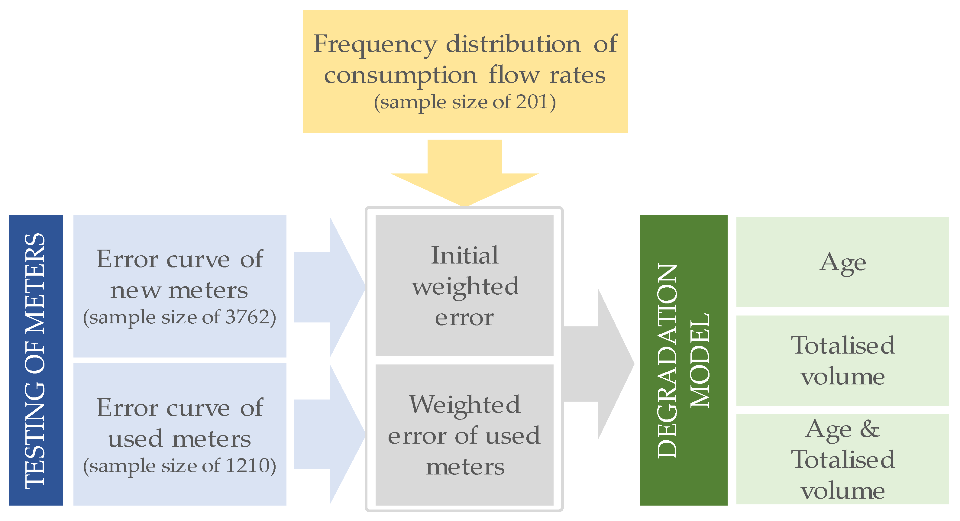
For a better understanding of the methodology followed and the amount of data used, Figure 1 shows the different stages comprising the analysis carried out and the relevant information associated with each one of them.
2.2. Water Consumption Flow Rates of Domestic Users
Water consumption flow rates from customers are not uniform throughout the day. Depending on the number and characteristic of the water appliances being used at each specific time, the flow rate passing through the meter may change. Therefore, when measuring water consumption from any user, water meters work under varying flow conditions. As defined by the error curve, the measuring errors of any water meter change depending on the flow rate passing through it. Consequently, two parameters are needed to calculate how much water is not registered by a meter when measuring the consumption of a specific user: (1) statistics about how much water is consumed at each flow rate (2) details on the error curve that provides information about the measuring errors at different flow rates. Information about the first parameter is summarized in the so-called water consumption pattern (a frequency distribution function of the consumption flow rates), which is built as a histogram that stratifies water consumption into several flow rate ranges. Examples of actual domestic consumption patterns in different countries can be found in Bowen et al. [29] and DeOreo el al. [30] in the USA, Beal and Stewart [31] in Australia, and Arregui et al. [10,16] in Spain. Other frequency distribution functions for particular types of customers can be found in Arregui et al. [32].
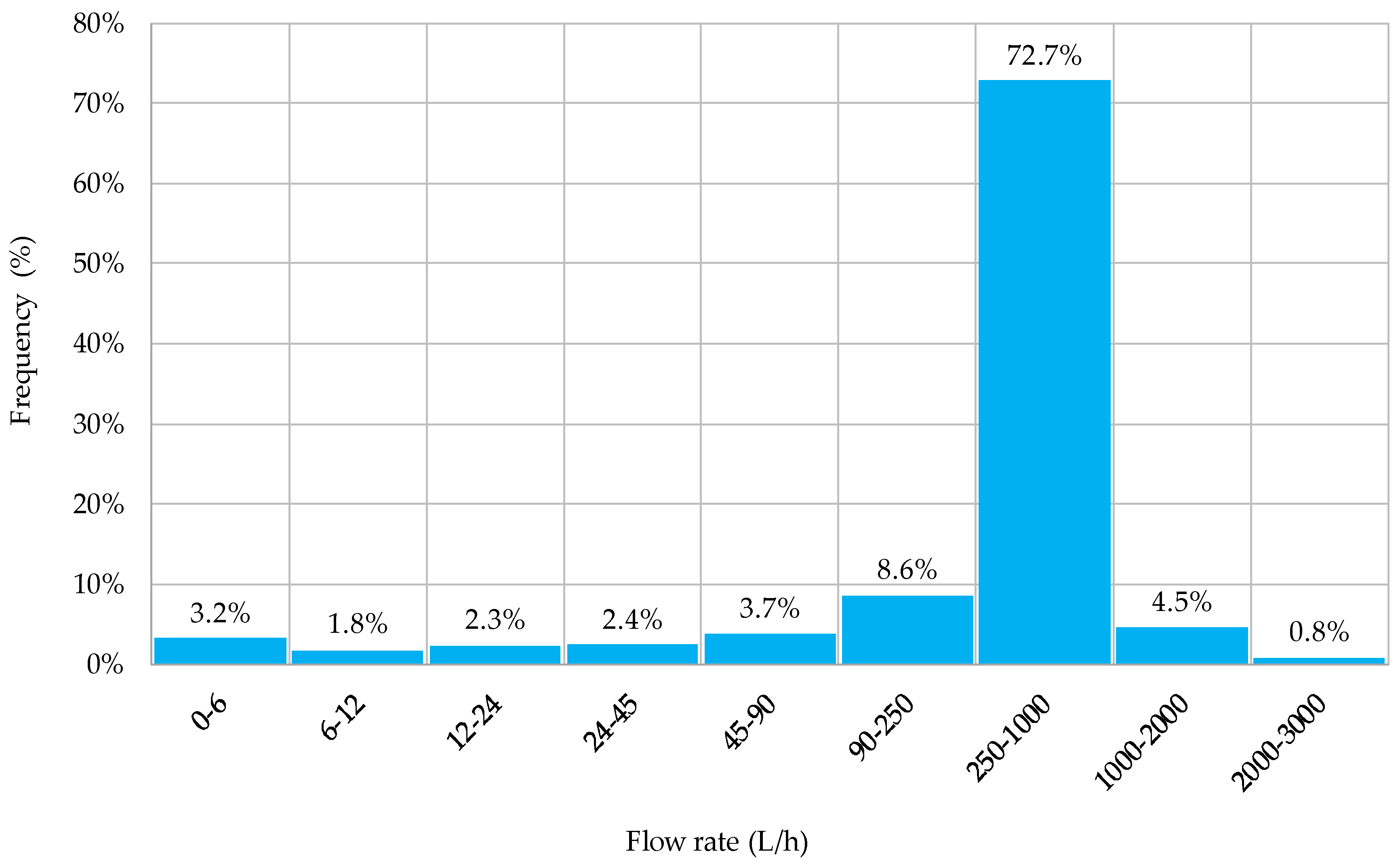
For the particular analysis conducted in this study, a frequency distribution of consumption flow rates (Figure 2) extracted from residential customers of one of the water supply systems managed by FACSA is used [26]. This frequency distribution was obtained by measuring, for a period of approximately two weeks, the water consumption of 201 domestic customers with a resolution of 0.1 L. The consumption data were recorded with a time resolution of 0.02 s. The oscillating piston water meters employed in the monitoring campaign were produced by ITRON (Aquadis) and the data-loggers used were manufactured by Sensus (Cosmos Data Logger). The fieldwork took place between November 2005 and April 2006. The methodology followed in this study is the same as described in Arregui et al. [16].
The obtained frequency distribution did not show a large percentage of volume consumed at low flows. In fact, on average, only 7.3% of the consumption took place at flow rates lower than 24 L/h, where domestic single-jet water meters may have most problems for measuring water volumes [13,19]. At higher flows, this percentage decreases and the amount of water consumed between 24 and 45 L/h represents only 2.4% of total consumption. According to the frequency distribution, most of the water usage, up to 72.7%, takes place between 250 and 1000 L/h. Finally, because of the characteristics of the households—mainly apartments located in residential buildings—the amount of water consumed above 2000 L/h is negligible, only 0.8%. The reason for this can be found in the sporadic overlapping of uses within the household and the limited consumption flow rate of the water appliances. Considering that according to the ISO 4064:2014-1, the overload flow rate of a typical domestic meter (with a permanent flow rate of 2.5 m3/h) is 3125 L/h, it is clear that most water consumption of the monitored users is well below the maximum capacity of any domestic meter. In other words, the meters typically installed for measuring water consumption in apartments are oversized considering the actual consumption flow rates of the users.
2.3. Testing Equipment and Procedures
Measuring errors of new and used meters were obtained by means of two different volumetric test benches, both having two calibrated probes of 10 L and 200 L and located in the laboratories of ITA and FACSA. For the particular case of domestic meters, the benches can fit up to 5 and 6 m respectively—which can be tested from 1 L/h up to 3125 L/h. The errors of the meters were obtained with the standing start and stop test method [33,34,35]. The 10 L probe was used to test the meters for flows up to 120 L/h; while the 200 L probe was used for flows higher than 120 L/h. The scale division of the probes was of 0.01 and 0.2 L, respectively, which represents 0.1% of the tested volume.
This means that the expanded uncertainty of the error tests conducted in this work was mainly driven by the resolution of the volume readings of the meters. For both meter types the smallest volume that could be read from the register was 0.05 L. This represents 0.5% when the test volume was 10 L and 0.025% when it was 200 L. All in all, the estimated test uncertainty was less than 0.2% for flow rates larger than 120 L/h and approximately 0.8% for tests equal or below 120 L/h.
When selecting the flow rates at which the meters should be tested, it is crucial to make a distinction between legal metrology tests and tests designed to establish the actual performance of the meters in the field, that is, the weighted error. In both cases, the criteria are completely different. For legal metrology, testing is mainly conducted to determine if the meters meet the metrological requirements at the flow rates specified by the standards. If the accuracy tests are limited to these flow rates it is extremely difficult to make a proper reconstruction of the error curve in the whole measuring range [32,36]. For this reason, and considering that the tests were conducted to establish the weighted error of the meters, the selection of flow rates had to take into consideration the need of obtaining an accurate representation of the performance at low flows [18,37,38,39]. This is the only scientific methodology that allows for a proper calculation of the weighted error of the meters. Considering this, the meters under analysis were tested at seven flow rates, four of which were at a flow rate equal or lower than 120 L/h. Also, both meter types underwent two slightly different sets of tests; one aimed at obtaining the initial metering performance before installation (Table 2) and the other conducted to verify the actual performance of the meters removed from the field (Tables 3–6). The main difference between both testing procedures was related to the order in which the meters were tested at the selected flow rates, the determination of the starting flow rate, and the magnitude of the largest flow rate.
2.4. Water Meter Sample Description
The presented work focused on two types of single-jet domestic water meters from different manufacturers (hereinafter called M_1 and M_2). Both types have an extra-dry register and a magnetic coupling between the turbine and the register. Other relevant technical and metrological characteristics of these meter types are described in Table 1. The initial weighted error of both types was calculated analysing a sample of 3762 new meters: 1068 corresponded to type M_1 and 2694 to M_2. The accuracy tests of new meters took place between 2008 and 2014. In addition to the extensive analysis conducted to the new meters, a stratified sample of 1210 m of the same two meter types under study was taken from the field. A total of 406 m of type M_1 and 804 m of type M_2 with different ages and volumes were analysed. The accuracy tests of the ageing meters were conducted between 2010 and 2015. A detailed stratification of meters by type, age and totalised volume can be found in Tables 3–6. In total, the research carried out has analysed the error curves at seven flow rates of 4972 m.
3. Results and Discussion
3.1. Error Curves
3.1.1. Error Curves of New Meters
Table 2 presents the average results of the accuracy tests conducted on the sample of new meters stratified by type. Except for a few exceptions, the errors obtained for both brands fall within the maximum permissible error tolerances allowed for their metrological class [2,40]. However, M_1 showed a poor metrological performance at the highest flow rates. This can be explained by the weakness of the magnetic coupling between the turbine and the register [16]. Some of the tested units presented an error greater than –60% at 3000 L/h. Nonetheless, this undesirable performance at the overload flow rate had a limited practical impact on the weighted error of the meters since the amount of water consumed around this flow is almost negligible (as defined by the frequency distribution of consumption flow rates in Figure 2). In this particular case, assuming a measuring error of 0% instead of –3.6% at 3000 L/h, the weighted error becomes 0.3% more positive.
The minimum flow rate of a Class B meter with a permanent flow rate of 1.5 m3/h is 30 L/h and the transitional flow rate is 120 L/h [40]. This means that for flow rates between 30 L/h and 120 L/h, the maximum permissible error is ±5% and for flow rates equal or above 120 L/h, the maximum allowable error is ±2%. In both cases, the average error of the sample within the measuring range, between 30 L/h and 3000 L/h, is positive except at the maximum flow rate of M_1 when some meters had a marked underperformance. In addition, the results presented in Table 2 show that the error curve of M_1 is slightly more positive than the error curve of M_2.
3.1.2. Error Curves of Ageing Meters
The average metering errors for different flow rates and ages are shown in Table 3 and Table 4. From these tables, it is clear that at medium and high flows, 750 L/h and above, the error variation is almost negligible for meter M_1 and small for M_2. However, at low flows, the measuring errors significantly increase (become more negative) with age. On the other hand, even though the starting flow rate of used meters was not tested in this study, the magnitude of the error at the lowest flow rate is negatively correlated with the value of the flow rate at which the impeller starts to move [41] and it can be used to estimate the starting flow. In other words, when meters become older, the starting flow rate is larger and the amount of water consumed below the starting flow rate rises. This implies that the rate at which the starting flow rate of a meter increases is strongly related to the rate at which the weighted error of a meter evolves with time.
Additional to this analysis, the average error curves were calculated by stratifying both meter types according to their totalised volume. The resulting errors for each flow rate and totalised volume group are shown in Table 5 and Table 6.
The errors obtained manifestly show that metrological performance degradation is more pronounced at low flows where single-jet meters have a strong tendency to under-register water consumption. At medium and high flows, 750 L/h and above, the average errors remain quite stable, especially for meter type M_1. The reason for this is that a number of units, 14 out of 406 of meter type M_1 and 40 out 804 of meter type M_2, showed an over-registration greater than +3% at flows 750 L/h and above. Moreover, three meters of each type presented an error of indication greater than +10%. This tendency of some single-jet meters to over-register water consumption under specific conditions has been reported by References [42,43] and partly compensates the negative errors that may appear in some units.
Finally, it was observed that the strength of the magnetic coupling of the older units of meter type M_2 (more than 5 years old) has significantly degraded and there is some slipping between the impeller and the register at high flows (Table 4 and Table 6). This behaviour can be easily identified in meters being more than 6 years old and having a large totalised volume, more than 3000 m3. The breakage of the magnetic coupling at high flows can produce a significant under-registration when measuring the water consumption of large water consumers. However, this is not significant for the type of domestic customer present in the water supply area (apartment located in residential buildings) which sporadically consumes water above 2000 L/h as shown in Figure 2.
3.2. Weighted Error of New Meters
The data obtained from the accuracy tests of the meters cannot be properly used unless the errors are combined with the associated consumption flow rates of the users (Figure 2) to calculate the weighted error. This indicator can be used as the initial reference to derive the degradation rate of the accuracy as a function of age or the totalised volume.
For both meter types and the used frequency distribution function of the consumption flow rates (Figure 2), the initial weighted error of the tested meters is close to −4%. This means that a newly installed single-jet water meter, of the tested types, is capable of registering approximately 96 out of 100 L consumed. This conclusion is in line with the results obtained from other researchers and clashes with the preconceived idea of some utility managers that a brand new meter can register 100% of the water consumed by the customers [23,25]. The inability of the meters studied to measure 100% of the water consumed by domestic users is mainly due to their limited performance at low flows. The starting flow rate, in both cases around 5 L/h (Table 2), is the threshold below which the meters do not register any consumption, that is, have a measuring error of −100%. Above this flow rate, the errors are negative and rapidly increase to values close to −5%. Measuring errors of the meters for flow rates above 30 L/h are close to 0% and produce a limited impact on the weighted error. More precisely, the initial weighted error obtained for M_1 was −3.5% while for M_2 the resulting weighted error was −3.9%. As expected, the differences in weighted errors between them are almost negligible and mainly driven by the slightly more positive error curve of M_1.
Following this calculation, the analysis described in the succeeding subsections refers to the evolution of the calculated weighted errors with age, totalised volume, or both parameters simultaneously.
3.3. Degradation Rate of the Weighted Error
3.3.1. Degradation Rate with Age
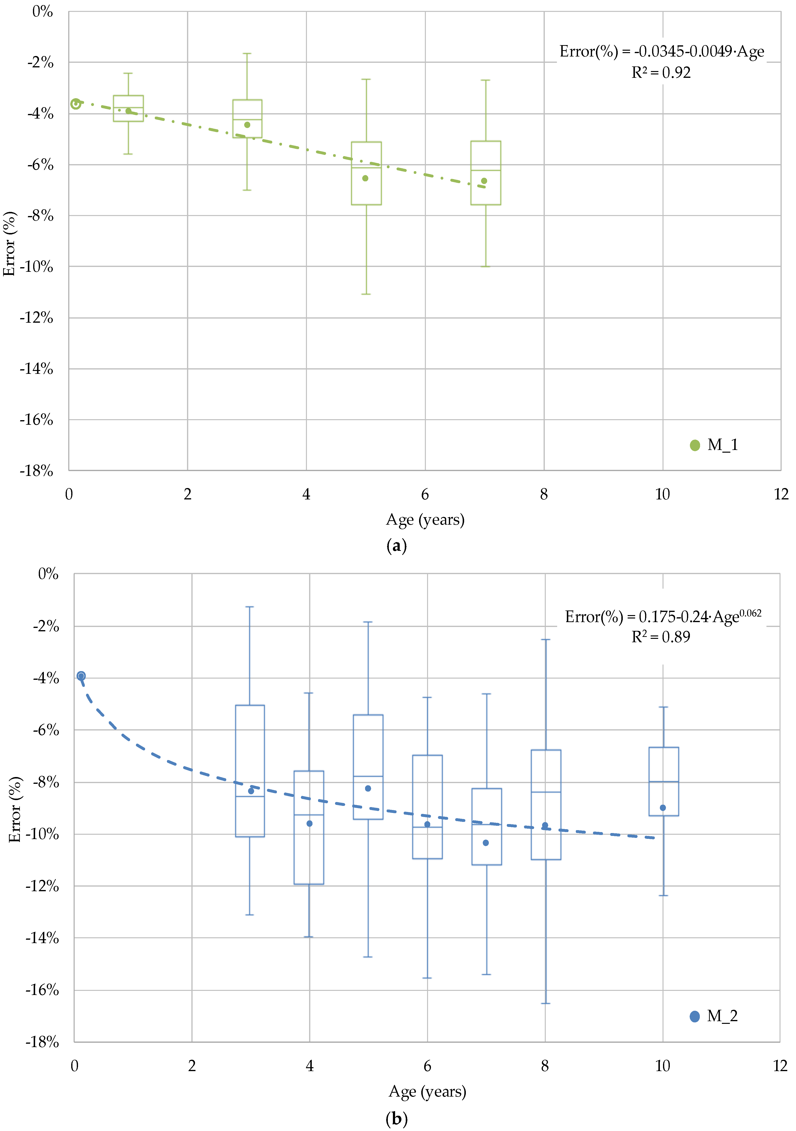
Figure 3 shows the degradation rate of the weighted error for both types against age. The number of meters tested of each one by age group is shown in Table 3 and Table 4.
Frequently, previous studies on meter degradation consider that the weighted error of domestic meters degrades linearly from an initial value [16,23,25,28,44,45]. Conversely, from the results presented in Figure 3, it is not obvious that a linear trend adequately represents the evolution of the weighted error with time. In the particular case of M_2, it seems that there is a quick initial degradation rate and after a few years, the weighted error tends to evolve at a much slower rate or even remain constant. On the contrary, the behaviour of meter type M_1 can be accurately described by a linear trend. In any case, from this graph, it is obvious that the measuring performance of meter M_2 is worse than the one obtained for M_1 at any age (except for brand new meters when the performance of both types are quite similar).
Additionally, when analysing the results presented in Figure 3, it should be noted that even though all units belonging to a specific meter type are considered to be the same, they can show significant manufacturing changes over time, not visible from the outside, that may have caused considerable behaviour discrepancies. At the time the study was conducted, more detailed information about these potential manufacturing changes was not available.
Overall, a regression model in the following form can describe how the weighted error, W. Error (%), evolves with age:
where age is expressed in years, E0(%) is the initial error, and the parameters A and B can be obtained by a regression analysis of the data. In the particular case of the linear regression commonly used by other authors in References [4,5,16,44], the parameter B would adopt a value of 1.
3.3.2. Degradation Rate with Totalised Volume
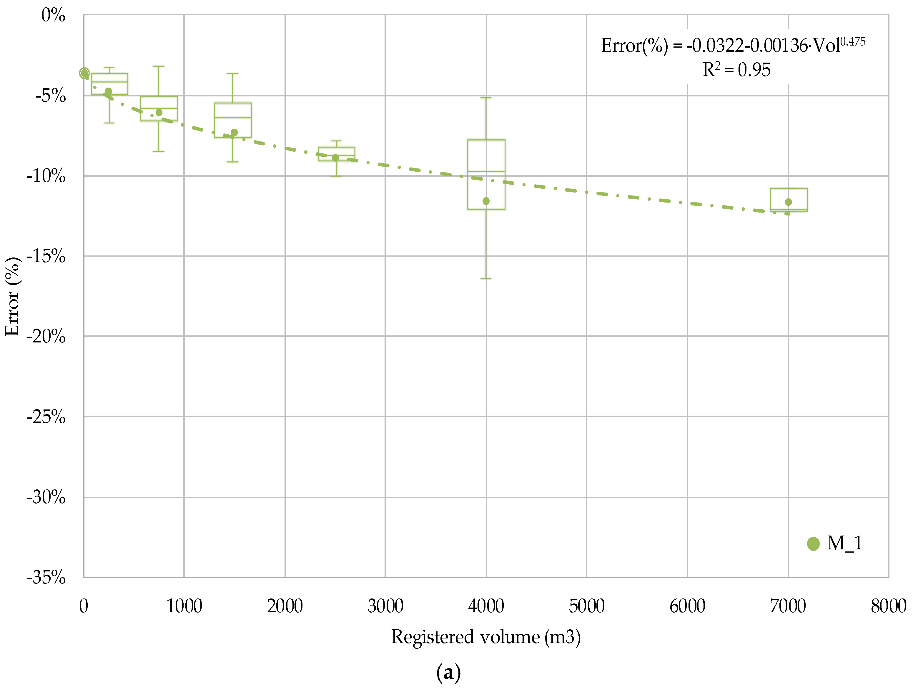
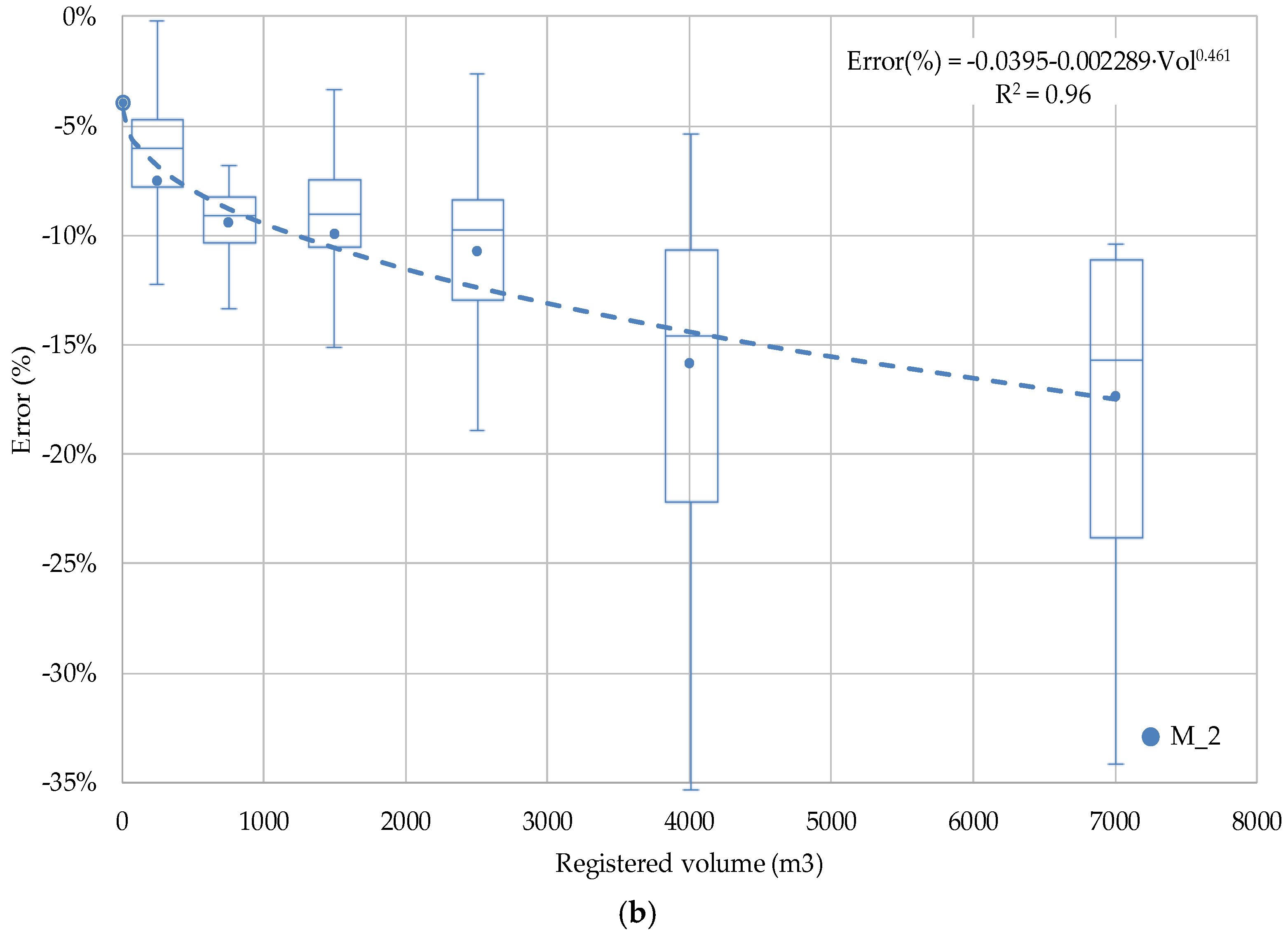
Figure 4 presents the weighted error trends of both meter types with respect the totalised volume. In this case, the R2 coefficients obtained are closer to 1 and the models proposed better explain the variability of the results. For both meter types, the mathematical regression that provided the best fitting to the data was not linear. Similarly, to what has been observed with the age of the meters, the average rate at which the meters degrades slow down as the meters register more water. Additionally, in this graph, it can be observed that the average performance of meter type M_2 is significantly worse than for M_1 for any totalised volume. This reinforces the idea that the initial error is not an appropriate parameter to select the most profitable water meter for the utility.
From the above, it has been concluded that a regression model in the form of
which can describe how the weighted error is related to the totalised volume of the meters (expressed in cubic meters).
3.3.3. Degradation Rate with Age and Totalised Volume
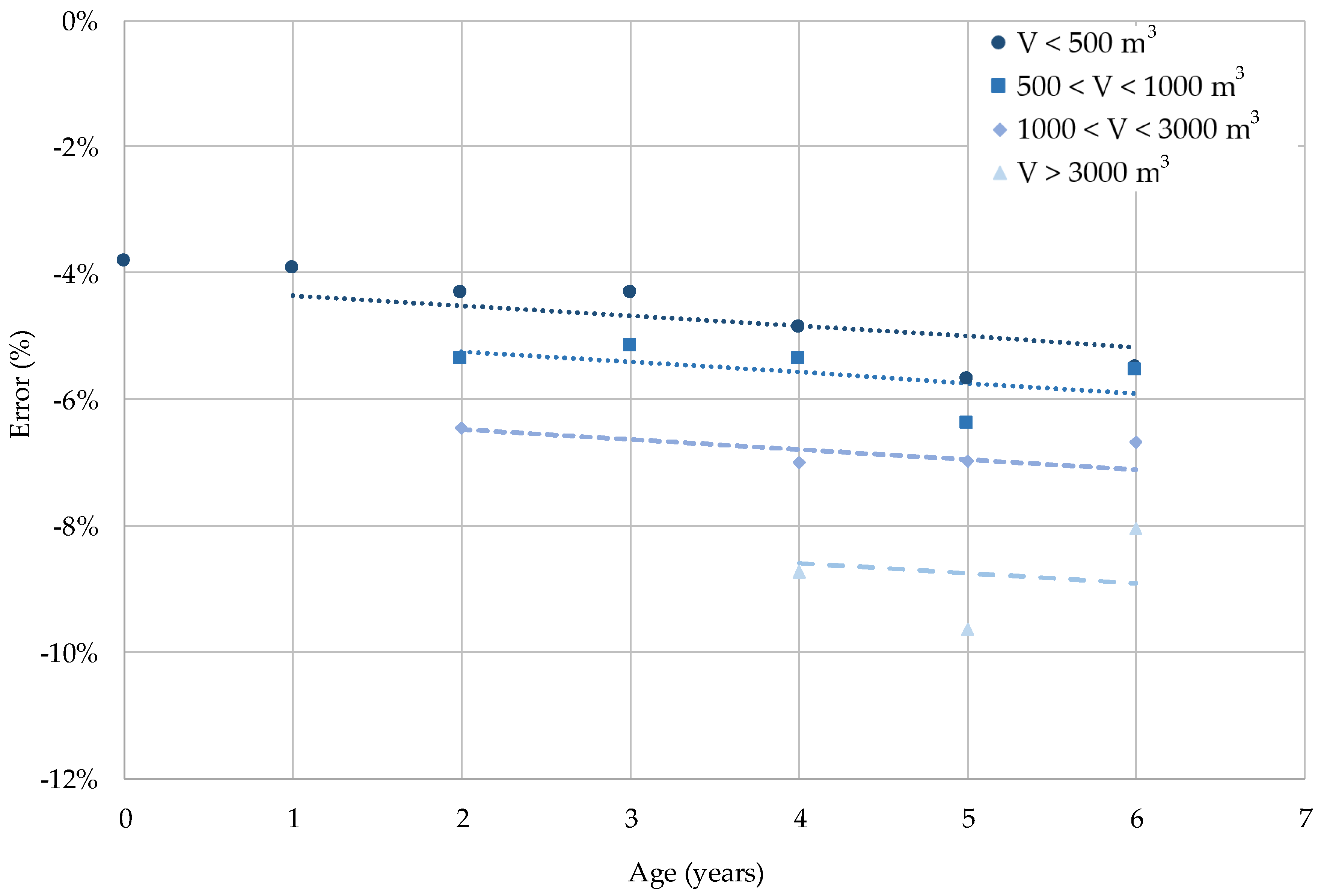
Figure 5 shows the weighted error plotted against age and totalised volume for meter type M_1. This figure allows for a better understanding of how age and totalised volume can affect the weighted error of a particular meter type. As can be seen, the dispersion of the error increases with the age and totalised volume of the meters. The overall tendency is that the meter error becomes more negative with both age and totalised volume. In the case of M_1, it was found that a linear regression could represent the degradation of the weighted errors with age for all the totalised volume ranges.
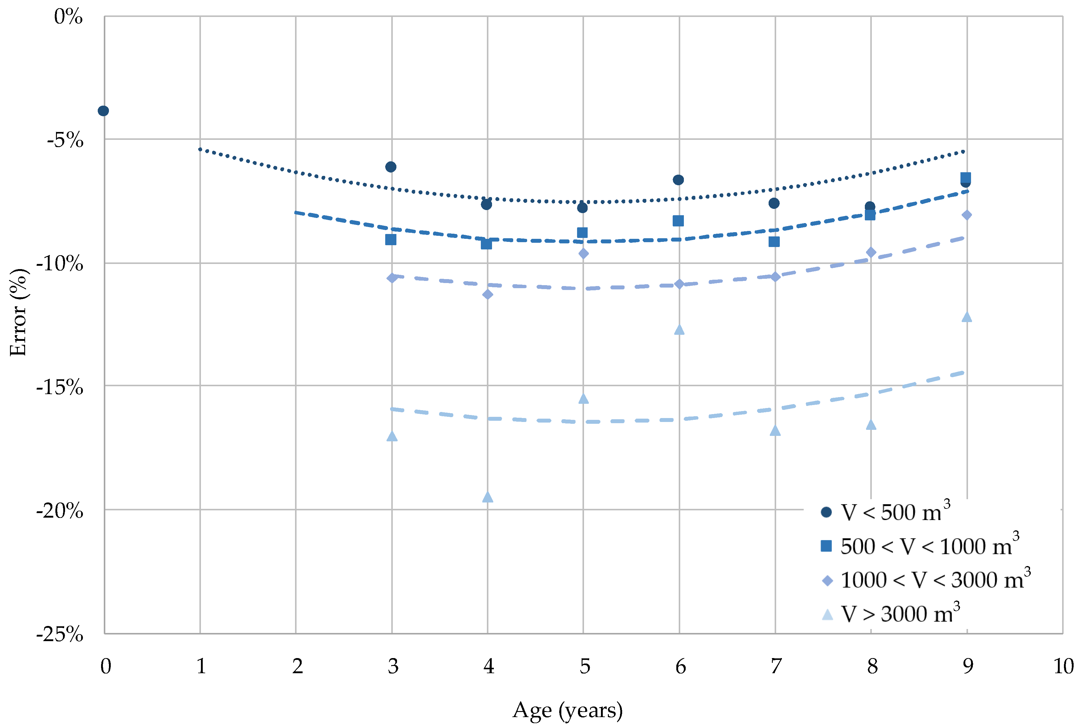
A similar analysis was conducted for meter type M_2. For this meter type, the sample size was larger (Table 1) and the evolution of the error with age and totalised volume did not follow a linear trend (Figure 6). For M_2 it was observed that older meters (more than 6 years old), independently of the totalised volume group, have slightly more positive errors than meters being between 2 and 5 years of age. This behaviour can be explained by the working principle of single-jet meters. Some of these meters have a slight tendency to over-register water consumption with the appearance of moderate calcium depositions [16,46]. Generally speaking, these depositions grow as meters become older but there are other parameters that can affect how fast they evolve, such as water quality, brass composition, working conditions, and so forth.
Consequently, this particular single-jet meter type seems to have a tendency to slightly improve its overall performance as it becomes older. In any case, the weighted error is considerably larger, for any age and totalised volume range, than for meter type M_1. In addition, it should be remarked that the oldest meter tested of M_1 type was only 7 years old and the improvement of meter type M_2 only became significant after this age.
3.3.4. Mathematical Degradation Model
A combined mathematical model that simultaneously takes into account age and totalised volume can be built using the results of the weighted error calculations made for the two meter types. The proposed degradation model should account simultaneously for both effects while maintaining a relative simplicity that makes it usable in practice. For this reason, the proposed non-linear combined degradation model adds (1) the initial weighted error of the meter type, E0(%), (2) a polynomial term accounting for the error due to age, and (3) a term accounting for the supplementary error due to the totalised volume. This theoretical model can be mathematically written in the following form:
where the age is expressed in years, the totalised volume in cubic meters and the parameters—A, B, C and D—can be obtained by conducting a non-linear regression of the available data (Statgraphics 9.0). A reliable figure for the initial error of the meter type, E0(%), can be derived from the results of the quality control tests conducted on new meters prior to installation. The regression parameters obtained for the two meter types under study are detailed in Table 7.
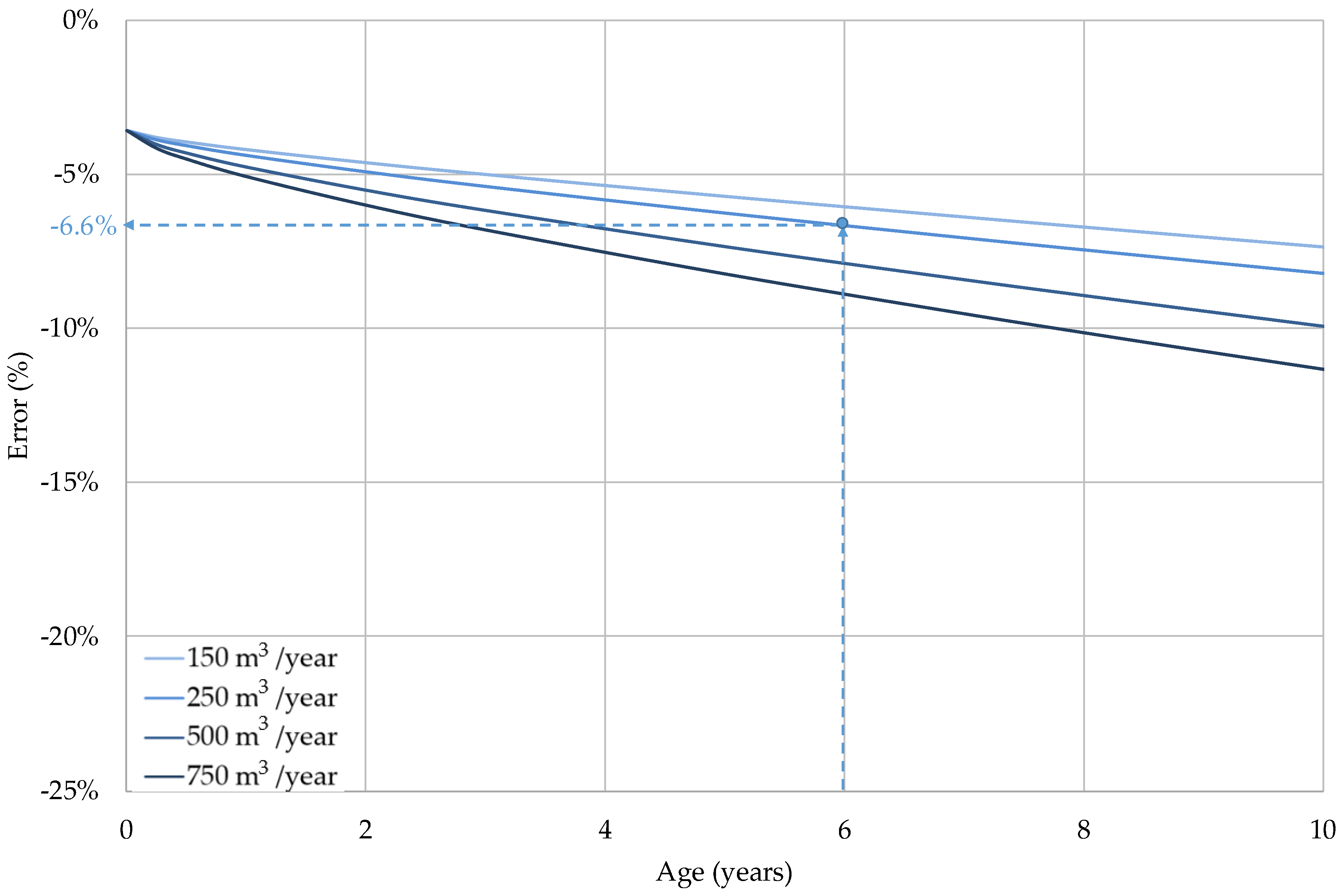
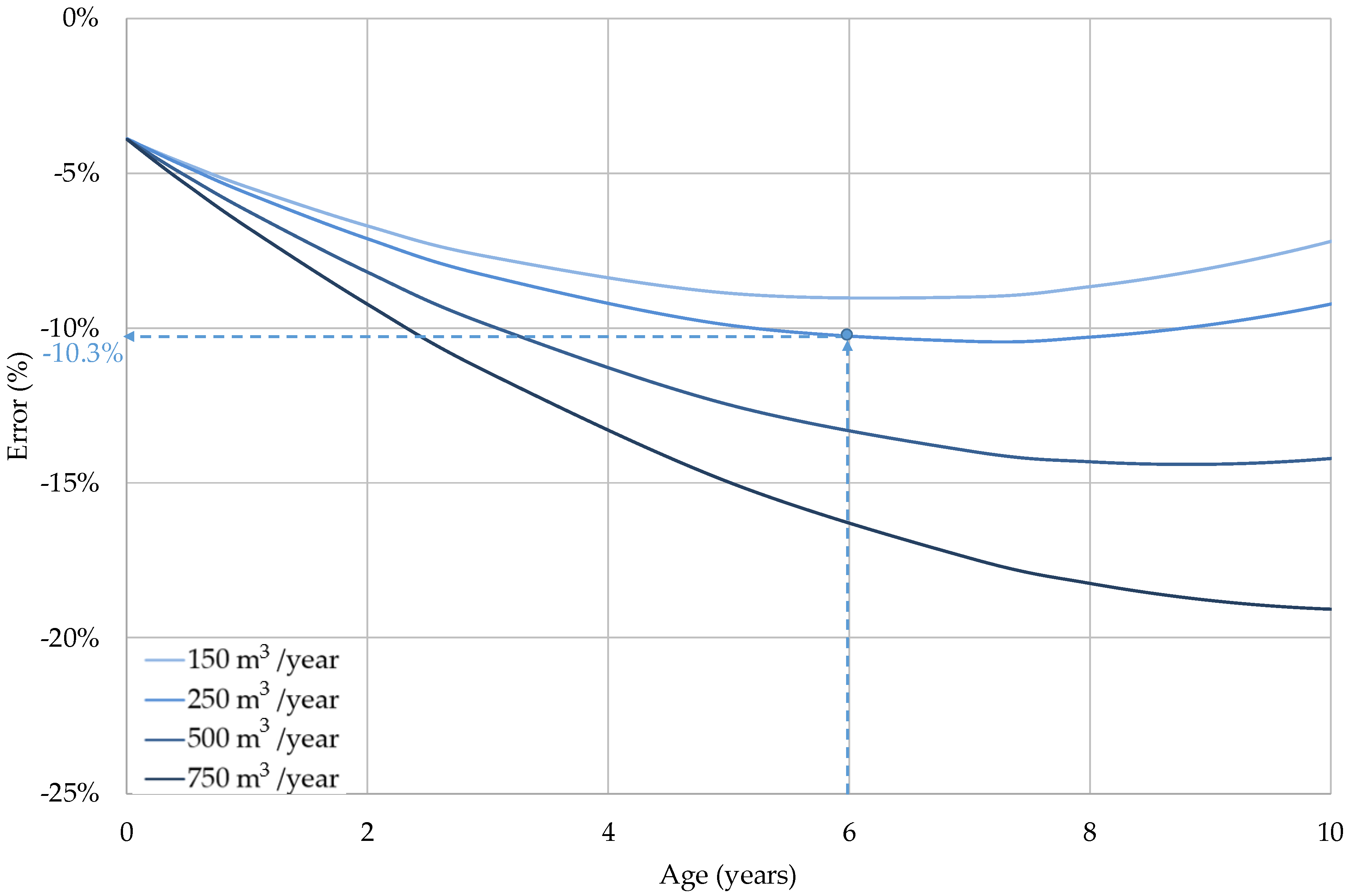
Figure 7 and Figure 8 present the expected evolution of the weighted error of both meter types, according to the degradation models obtained from the tests, for different ages and annual consumption rates. For example, from Table 7 and Equation (3) it is possible to obtain the estimated error of a meter M_1 or M_2 being 6 years old and measuring water consumption of a customer using an average of 250 m3/year. In this case, the totalised volume after 6 years would be 1500 m3 and the resulting weighted errors are −6.6% for meter type M_1 and −10.3% for meter type M_2. The same results can be obtained using Figure 7 and Figure 8.
Table 8 compares the weighted errors, calculated for meters of being 6 years old, using the three degradation models proposed. The improvement in the estimation of the weighted error derived from using a combined multivariate model, in comparison with simpler univariate models, is more significant for M_2 than for M_1. The reason for this can be found in the fact that totalised volume seems to have a more limited effect on M_1 (Figure 5 versus Figure 6). Also, the results obtained from the model using the totalised volume are significantly closer to the ones calculated from the multivariate model than the ones derived from the model using age as the driver for the weighted error degradation.
4. Conclusions
This paper describes the results obtained from a work that was conducted during the past years in coordination with a water utility in Spain. The purpose of the study was to obtain the real degradation rates of the weighted error for two types of single-jet domestic water meters that are being used by FACSA in several water distribution systems and shows if a procurement selection procedure should not be mainly based on the initial errors of the meters.
The analysis of the weighted error of the meters tested shows that the usual assumption, which considers a linear degradation with age or totalised volume, is only acceptable in some cases. In other cases, like for one of the meters under study, this simplification is not acceptable. This work proposes a modified regression model to estimate more accurately the evolution of the weighted error with age and totalised volume as single drivers.
Another frequent simplification when estimating the measuring error of installed meters is to carry out a univariate regression analysis, using age or totalised volume, of the degradation of the weighted error. These models consider only one variable as the drivers of the weighted error. However, univariate regression models may not be accurate enough to establish the real performance of ageing meters. For example, a degradation model that only takes into account age will provide the exact same estimation for the weighted error of meters installed in customers with different consumption rates. However, the presented work has found that there are significant differences in the weighted error of meters having the same age and different totalised volume.
To improve the estimation of the actual performance of the meters this paper has presented a multivariate analysis of the weighted error degradation rates. The aim is to quantify the combined effect of age and totalised volume on the weighted error of the meters. For this purpose, a non-linear model—applicable to the meter types under analysis—that takes into account the initial error of the meters and the simultaneous impact of age and totalised volume has been derived. The proposed degradation model calculates more accurately the weighted error of the meters measuring the consumption of those customers having extremely low or large consumption rates.
It has been found that, for the meters under study, the differences between the proposed multivariate model and the model using the totalised volume are smaller than the ones found for the model using the age of the meters as the driver for the weighted error degradation. Following this, it can be concluded that for the meters analysed, the totalised volume can provide a better approximation than age.
Finally, it is important to highlight that the results obtained for the particular meter types tested cannot be extrapolated to other water utilities as the parameters that may affect the weighted error of ageing meters may differ from those present in the water supply studied. In addition, in order to obtain an accurate approximation of the measuring errors of installed meters, all meter types need to be tested and analysed. Two meter types can behave completely different in a specific water system and the same meter type can present dissimilar ageing processes in two different water systems.
Author Contributions
Methodology conception and definition: F.J.A. Meter testing, data gathering and analysis of the accuracy tests results: J.S. and L.P.-J. Data analysis of the weighted error: F.J.A. and F.J.G. Water consumption pattern of residential users: F.J.A. and F.J.G. All authors contributed to the preparation of the manuscript and approved it.
Funding
This study has received funding from the IMPADAPT project/CGL2013-48424-C2-1-R from the Spanish ministry MINECO with European FEDER funds.
Conflicts of Interest
The authors declare no conflict of interest.
References
- Lambert, A.O. International report: Water losses management and techniques. Water Sci. Technol. Water Supply 2002, 2, 1–20. [Google Scholar]
- International Organization for Standardization (ISO). ISO 4064-1:2014—Water Meters for Cold Potable Water and Hot Water—Part 1: Metrological and Technical Requirements; ISO: Geneva, Switzerland, 2014. [Google Scholar]
- International Organization for Standardization (ISO). ISO 4064-3:2014—Water Meters for Cold Potable Water and Hot Water—Part 3: Test Report Format; ISO: Geneva, Switzerland, 2014. [Google Scholar]
- Mbabazi, D.; Banadda, N.; Kiggundu, N.; Mutikanga, H.; Babu, M. Determination of domestic water meter accuracy degradation rates in Uganda. J. Water Supply Res. Technol. 2015, 64, 486–492. [Google Scholar] [CrossRef]
- Mutikanga, H.; Sharma, S.; Vairavamoorthy, K. Investigating water meter performance in developing countries: A case study of Kampala, Uganda. Water SA 2011, 37, 567–574. [Google Scholar] [CrossRef]
- Fontanazza, C.M.; Freni, G.; la Loggia, G.; Notaro, V.; Puleo, V. A composite indicator for water meter replacement in an urban distribution network. Urban Water J. 2012, 9, 419–428. [Google Scholar] [CrossRef]
- Fontanazza, C.M.; Notaro, V.; Puleo, V.; Freni, G. The apparent losses due to metering errors: A proactive approach to predict losses and schedule maintenance. Urban Water J. 2015, 12, 229–239. [Google Scholar] [CrossRef]
- Mutikanga, H.E.; Sharma, S.; Vairavamoorthy, K. Water loss management in developing countries: Challenges and prospects. Am. Water Works Assoc. J. 2009, 101, 57–68. [Google Scholar] [CrossRef]
- Mutikanga, H.E.; Sharma, S.K.; Vairavamoorthy, K. Assessment of apparent losses in urban water systems. Water Environ. J. 2011, 25, 327–335. [Google Scholar] [CrossRef]
- Díaz, I.; Flores, J. Precisión de la Medida de los Consumos Individuales de Agua en la Comunidad de Madrid; Canal de Isabel II: Madrid, Spain, 2010; ISBN 978-8-49-364453-6. [Google Scholar]
- Larraona, G.S.; Rivas, A.; Ramos, J.C. Computational modeling and simulation of a single-jet water meter. J. Fluids Eng. 2008, 130, 051102. [Google Scholar] [CrossRef]
- Zhen, W.; Tao, Z. Computational study of the tangential type turbine flowmeter. Flow Meas. Instrum. 2008, 19, 233–239. [Google Scholar] [CrossRef]
- Rizzo, A.; Cilia, J. Quantifying Meter Under-Registration Caused by the Ball Valves of Roof Tanks (for Indirect Plumbing Systems). In Proceedings of the IWA Leakage Conference ‘Leakage 2005’, Halifax, NS, Canada, 12–14 September 2005; pp. 1–12. [Google Scholar]
- De Marchis, M.; Fontanazza, C.M.; Freni, G.; La Loggia, G.; Notaro, V.; Puleo, V. A mathematical model to evaluate apparent losses due to meter under-registration in intermittent water distribution networks. Water Sci. Technol. Water Supply 2013, 13, 914–923. [Google Scholar] [CrossRef]
- Criminisi, A.; Fontanazza, C.M.; Freni, G.; La Loggia, G. Evaluation of the apparent losses caused by water meter under-registration in intermittent water supply. Water Sci. Technol. 2009, 60, 2373–2382. [Google Scholar] [CrossRef] [PubMed]
- Arregui, F.J.; Cabrera, E.J.; Cobacho, R. Integrated Water Meter Management; IWA Publishing: London, UK, 2006. [Google Scholar]
- Bowen, P.T.; Harp, J.F.; Entwistle, J.M., Jr.; Shoeleh, M. Evaluating Residential Water Meter Performance; Prepared for AWWA Research Foundation—Version details—Trove; AWWA Research Foundation and American Water Works Association: Denver, CO, USA, 1991.
- Richards, G.L.; Johnson, M.C.; Barfuss, S.L. Apparent losses caused by water meter inaccuracies at ultralow flows. J. Am. Water Works Assoc. 2010, 102, 123–132. [Google Scholar] [CrossRef]
- Stoker, D.M.; Barfuss, S.L.; Johnson, M.C. Flow measurement accuracies of in-service residential water meters. J. Am. Water Works Assoc. 2012, 104, 33. [Google Scholar] [CrossRef]
- Pasanisi, A. Aide à la Décision Dans la Gestion des Parcs de Compteurs d’eau Potable. Ph.D. Thesis, ENGREF (AgroParisTech), Paris, France, 2004. [Google Scholar]
- Shields, D.J.; Barfuss, S.L.; Johnson, M.C. Revenue recovery through meter replacement. J. Am. Water Works Assoc. 2012, 104, 69–70. [Google Scholar] [CrossRef]
- Arregui, F.J.; Cobacho, R.; Cabrera, E., Jr.; Espert, V. A graphical method to calculate the optimum replacement period of water meters. J. Water Resour. Plan. Manag. 2011, 137, 143–146. [Google Scholar] [CrossRef]
- Yee, M.D. Economic analysis for replacing residential meters. Am. Water Works Assoc. J. 1999, 91, 72–77. [Google Scholar] [CrossRef]
- Davis, S. Residential Water Meter Replacement Economics. In Proceedings of the IWA Leakage Conference ‘Leakage 2005’, Halifax, NS, Canada, 12–14 September 2005; pp. 1–10. [Google Scholar]
- Allender, H. Determining the economical optimum life of residential water meters. Water Eng. Manag. 1996, 143, 20–24. [Google Scholar]
- Gavara, F. Estudio del Comportamiento Metrológico de los Contadores en Abastecimientos de Agua. Optimización de su Gestión para la Reducción de las Pérdidas Comerciales. Ph.D. Thesis, Universitat Politècnica de València, Valencia, Spain, 2015. [Google Scholar]
- Arregui, F.J. Meter Error Calculator. Available online: http://personales.upv.es/farregui/ (accessed on 21 March 2018).
- Hill, C.; Davis, S.E. Economics of Domestic Residential Water Meter Replacement Based on Cumulative Volume. In Proceedings of the AWWA Annual Conference, San Francisco, CA, USA, 12–16 June 2005. [Google Scholar]
- Bowen, P.T.; Association, A.W.W.; Foundation, A.R. Residential Water Use Patterns; The Foundation and American Water Works Association: Denver, CO, USA, 1993. [Google Scholar]
- Deoreo, W.B.; Mayer, P.W.; Dziegielewski, B.; Kiefer, J.C. Residential End Uses of Water, Version 2 (4309B); The Water Research Foundation: Denver, CO, USA, 2016. [Google Scholar]
- Beal, C.; Stewart, R.A. South East Queensland Residential End Use Study: Final Report. Urban Water Security Research Alliance Technical Report No. 47, City East, Australia. 2011. Available online: http://www.urbanwateralliance.org.au/publications/UWSRA-tr47.pdf (accessed on 7 May 2018).
- Arregui, F.J.; Cabrera, E.; Cobacho, R.; García-Serra, J. Reducing Apparent Losses Caused by Meters Inaccuracies. Technology 2006, 1, wpt2006093. [Google Scholar] [CrossRef]
- Spitzer, D.W. Flow Measurement: Practical Guides for Measurement and Control; The Instrumentation, Systems, and Automation Society (ISA): Research Triangle Park, NC, USA, 2001. [Google Scholar]
- Paton, R. Calibration and Standards in Flow. In Handbook of Measuring System Design; John Wiley & Sons, Ltd.: Hoboken, NJ, USA, 2005. [Google Scholar]
- ISO. ISO 4064-2:2014—Water Meters for Cold Potable Water and Hot Water—Part 2: Test Methods; ISO: Geneva, Switzerland, 2014. [Google Scholar]
- Arregui, F.J.; Martinez, B.; Soriano, J.; Parra, J.C. Tools for Improving Decision Making in Water Meter Management. In Proceedings of the 5th IWA Water Loss Reduction Specialist Conference, Cape Town, South Africa, 26–30 April 2009; pp. 225–232. [Google Scholar]
- Barfuss, S.L. Flow Meter Accuracy. In Proceedings of the American Council for an Energy-Efficient Economy (ACEEE), Berkeley, CA, USA, 10–12 May 2011. [Google Scholar]
- Barfuss, S.L.; Johnson, M.C.; Neilsen, M.A. Accuracy of In-Service Water Meters at Low and High Flow Rates; Water Research Foundation: Denver, CO, USA, 2011. [Google Scholar]
- Sumrak, M.L.; Johnson, M.C.; Barfuss, S.L. Comparing Low Flow Accuracy of Mechanical and Electronic Meters. J. Am. Water Works Assoc. 2016, 108, E327–E334. [Google Scholar] [CrossRef]
- ISO 4064-1:1993—Measurement of Water Flow in Closed Conduits—Meters for Cold Potable Water—Part 1: Specifications. Available online: https://www.iso.org/standard/9772.html (accessed on 20 March 2018).
- Arregui, F.J.; Palau, C.V.; Gascón, L.; Peris, O. Evaluating domestic water meter accuracy. A case study. Pumps Electromech. Devices Syst. Appl. Urban Water Manag. 2003, 1, 343. [Google Scholar]
- Diaz, I.; Flores, J. Accurate Assessment of under Metering in MADRID Water Supply. In Proceedings of the 5th IWA Specialist Conference on Efficient Use and Management of Urban Water (Efficient 2009), Sydney, Australia, 25–28 October 2009. [Google Scholar]
- Male, J.W.; Noss, R.R.; Moore, I.C. Identifying and Reducing Losses in Water Distribution Systems; Noyes Publications: Park Ridge, NJ, USA, 1985. [Google Scholar]
- Mukheibir, P.; Stewart, R.A.; Giurco, D.P.; Halloran, K.O. Understanding non-registration in domestic water meters: Implications for meter replacement strategies. Water J. 2012, 39, 95–100. [Google Scholar]
- Szilveszter, S.; Beltran, R.; Fuentes, A. Performance analysis of the domestic water meter park in water supply network of Ibarra, Ecuador. Urban Water J. 2017, 14, 85–96. [Google Scholar] [CrossRef]
- Arregui, F.J.; Cabrera, E.J.; Cobacho, R.; García-Serra, J. Key factors affecting water meter accuracy. In Proceedings of the IWA Leakage Conference ‘Leakage 2005’, Halifax, NS, Canada, 12–14 September 2005; pp. 1–10. [Google Scholar]
Figure 1.
The diagram of the methodology used.

Figure 2.
The frequency distribution for the consumption flow rates of the monitored residential users.
Figure 2.
The frequency distribution for the consumption flow rates of the monitored residential users.

Figure 3.
The degradation rate of the weighted error with age: (a) meter M_1; (b) meter M_2.

Figure 4.
The degradation rate of the weighted error with totalised volume: (a) meter M_1; (b) meter M_2.
Figure 4.
The degradation rate of the weighted error with totalised volume: (a) meter M_1; (b) meter M_2.


Figure 5.
The degradation rate of the weighted error with age and totalised volume (meter M_1).

Figure 6.
The degradation rate of the weighted error with age and totalised volume (meter M_2).

Figure 7.
The degradation of the weighted error with age for different annual consumption rates (meter M_1).
Figure 7.
The degradation of the weighted error with age for different annual consumption rates (meter M_1).

Figure 8.
The degradation of the weighted error with age for different annual consumption rates (meter M_2).
Figure 8.
The degradation of the weighted error with age for different annual consumption rates (meter M_2).


Table 1.
The technical and metrological characteristics of the meters sample.
| Meter Type | Tech. | Class | Standard | Qpermanent (m3/h) | Length (mm) | Sample—New Meters | Sample—Used Meters |
|---|---|---|---|---|---|---|---|
| M_1 | Single-Jet | B | ISO4064:1993 | 1.5 | 115 | 1068 | 406 |
| M_2 | Single-Jet | B | ISO4064:1993 | 1.5 | 115 | 2694 | 804 |
Table 2.
The average starting flow rate and error tolerance (%) of indication for each meter type.
| Meter | Sample Size | Qstart (L/h) | 15 L/h | 30 L/h | 60 L/h | 120 L/h | 600 L/h | 1500 L/h | 3000 L/h |
|---|---|---|---|---|---|---|---|---|---|
| M_1 | 1068 | 5.3 | −8.9 | 1.5 | 1.3 | 1.5 | 1.5 | 1.3 | −3.6 |
| M_2 | 2694 | 5.3 | −8.4 | 3.3 | 2.7 | 0.9 | 0.8 | 0.6 | 0.5 |
| ISO 4064 Error tolerance | N/A | ±5 | ±5 | ±2 | ±2 | ±2 | ±2 | ||
Table 3.
The average error of indication (%) of meter type M_1 classified by age.
| Age (years) | Meters Tested | 15 L/h | 30 L/h | 60 L/h | 120 L/h | 750 L/h | 1500 L/h | 2750 L/h |
|---|---|---|---|---|---|---|---|---|
| 1–2 | 79 | −12.2 | 0.9 | 1.3 | 1.4 | 1.1 | 0.9 | 0.3 |
| 3–4 | 96 | −22.3 | −0.8 | 1.3 | 1.2 | 0.9 | 0.7 | 0.1 |
| 5–6 | 114 | −49.1 | −14.3 | −4.7 | −1.2 | −0.4 | 0.3 | −0.2 |
| >7 | 117 | −35.2 | −8.1 | −2.5 | −0.7 | −0.3 | −0.4 | −1.0 |
Table 4.
The average error of indication (%) of meter type M_2 classified by age.
| Age (years) | Meters Tested | 15 L/h | 30 L/h | 60 L/h | 120 L/h | 750 L/h | 1500 L/h | 2750 L/h |
|---|---|---|---|---|---|---|---|---|
| 3 | 62 | −73.0 | −24.5 | −8.1 | −4.5 | −1.8 | −1.7 | −1.4 |
| 4 | 37 | −87.5 | −39.4 | −10.6 | −4.3 | −1.7 | −1.5 | −1.2 |
| 5 | 161 | −53.0 | −22.0 | −8.8 | −4.7 | −2.3 | −2.1 | −1.4 |
| 6 | 16 | −68.9 | −16.3 | −4.6 | −3.1 | −1.7 | −1.2 | −6.4 |
| 7 | 133 | −53.4 | −17.8 | −8.0 | −6.0 | −3.8 | −3.4 | −5.4 |
| 8–9 | 162 | −61.2 | −20.8 | −9.0 | −5.5 | −2.7 | −2.3 | −6.2 |
| >10 | 233 | −55.7 | −14.6 | −5.4 | −3.8 | −2.1 | −4.0 | −7.4 |
Table 5.
The average error of indication (%) of meter type M_1 classified by totalised volume.
| Total. Volume (m3) | Meters Tested | 15 L/h | 30 L/h | 60 L/h | 120 L/h | 750 L/h | 1500 L/h | 2750 L/h |
|---|---|---|---|---|---|---|---|---|
| 0–500 | 206 | −19.3 | −0.5 | 0.7 | 1.3 | 0.8 | 0.7 | 0.1 |
| 500–1000 | 89 | −30.6 | −5.4 | −0.7 | 0.5 | 0.4 | 0.1 | −0.4 |
| 1000–2000 | 67 | −40.8 | −10.2 | −3.3 | −0.5 | 0.1 | −0.2 | −0.7 |
| 2000–3000 | 23 | −69.9 | −14.7 | −2.5 | −0.9 | −0.3 | −0.4 | −0.8 |
| 3000–5000 | 14 | −87.7 | −44.7 | −19.0 | −15.2 | −7.7 | 0.2 | −1.0 |
| >5000 | 7 | −77.1 | −42.8 | −21.3 | −5.9 | −1.3 | −1.4 | −1.4 |
Table 6.
The average error of indication (%) of meter type M_2 classified by totalised volume.
| Total. Volume (m3) | Meters Tested | 15 L/h | 30 L/h | 60 L/h | 120 L/h | 750 L/h | 1500 L/h | 2750 L/h |
|---|---|---|---|---|---|---|---|---|
| 0–500 | 201 | −35.8 | −11.4 | −4.6 | −2.6 | 0.3 | 0.4 | −0.7 |
| 500–1000 | 190 | −50.8 | −10.9 | −4.1 | −2.5 | −1.6 | −1.2 | −1.2 |
| 1000–2000 | 262 | −64.3 | −15.9 | −4.0 | −2.5 | −1.4 | −2.2 | −3.9 |
| 2000–3000 | 106 | −82.8 | −32.1 | −10.4 | −4.5 | −1.7 | −2.9 | −8.0 |
| 3000–5000 | 35 | −94.4 | −65.8 | −26.9 | −12.6 | −3.9 | −3.7 | −20.5 |
| >5000 | 10 | −97.6 | −62.7 | −29.4 | −15.0 | −4.5 | −11.8 | −21.4 |
Table 7.
The regression parameters values of the proposed equation for the two meter types under study.
Table 7.
The regression parameters values of the proposed equation for the two meter types under study.
| Parameter | Meter M_1 | Meter M_2 |
|---|---|---|
| E0 | −3.49 | −3.91 |
| A | −0.152 | −1.313 |
| B | −0.00149 | 0.131 |
| C | −0.0174 | −0.00291 |
| D | 0.657 | 0.959 |
Table 8.
The comparison of the three degradation models proposed for meters being 6 years old.
| Model | Meter M_1 Totalised Volume | Meter M_2 Totalised Volume | ||||
|---|---|---|---|---|---|---|
| 900 m3 | 1500 m3 | 4500 m3 | 900 m3 | 1500 m3 | 4500 m3 | |
| Age | −6.4% | −6.4% | −6.4% | −9.3% | −9.3% | −9.3% |
| Totalised volume | −6.7% | −7.6% | −10.6% | −9.2% | −10.6% | −15.0% |
| Age & Totalised volume | −6.0% | −6.6% | −8.6% | −9.0% | −10.3% | −16.3% |
© 2018 by the authors. Licensee MDPI, Basel, Switzerland. This article is an open access article distributed under the terms and conditions of the Creative Commons Attribution (CC BY) license (http://creativecommons.org/licenses/by/4.0/).
Share and Cite
MDPI and ACS Style
Arregui, F.J.; Gavara, F.J.; Soriano, J.; Pastor-Jabaloyes, L. Performance Analysis of Ageing Single-Jet Water Meters for Measuring Residential Water Consumption. Water 2018, 10, 612. https://doi.org/10.3390/w10050612
AMA Style
Arregui FJ, Gavara FJ, Soriano J, Pastor-Jabaloyes L. Performance Analysis of Ageing Single-Jet Water Meters for Measuring Residential Water Consumption. Water. 2018; 10(5):612. https://doi.org/10.3390/w10050612
Chicago/Turabian StyleArregui, Francisco J., Francesc J. Gavara, Javier Soriano, and Laura Pastor-Jabaloyes. 2018. "Performance Analysis of Ageing Single-Jet Water Meters for Measuring Residential Water Consumption" Water 10, no. 5: 612. https://doi.org/10.3390/w10050612
Note that from the first issue of 2016, this journal uses article numbers instead of page numbers. See further details here.