Application of a Steady Meandering River with Piers Using a Lattice Boltzmann Sub-Grid Model in Curvilinear Coordinate Grid

Abstract

A sub-grid multiple relaxation time (MRT) lattice Boltzmann model with curvilinear coordinates is applied to simulate an artificial meandering river. The method is based on the D2Q9 model and standard Smagorinsky sub-grid scale (SGS) model is introduced to simulate meandering flows. The interpolation supplemented lattice Boltzmann method (ISLBM) and the non-equilibrium extrapolation method are used for second-order accuracy and boundary conditions. The proposed model was validated by a meandering channel with a 180° bend and applied to a steady curved river with piers. Excellent agreement between the simulated results and previous computational and experimental data was found, showing that MRT-LBM (MRT lattice Boltzmann method) coupled with a Smagorinsky sub-grid scale (SGS) model in a curvilinear coordinates grid is capable of simulating practical meandering flows.

1. Introduction

Derived from the Lattice Gas Automata (LGA) [1,2], the single relaxation method (called the lattice Bhatnagar Gross Krook (LBGK) method) [3,4] is a promising and powerful tool for computational fluid dynamics. It has also been successfully applied to simulate various of flow problems, such as free surface flow [5], advection and dispersion problems [6], multiphase fluids [7,8], and shallow water flows [9,10]. However, numerical instability is one of problems of the LBGK method, especially when the Reynolds number is high or the viscosity is low [11,12]. The multiple relaxation time (MRT) lattice Boltzmann method was proposed and developed [13,14,15] to overcome these shortcomings; by establishing a model on moment space rather than on discrete space, different relaxation times can be chosen for different moments, which leads to an improvement in the stability of the LBGK method [15].

Standard lattice Boltzmann method (LBM) is restricted to regular lattices, which is limits the simulation of curved and complex natural rivers. One way to solve this problem is to use nonuniform lattices. In recent years, different methods have been developed to extend the LBM on a nonuniform mesh, including the interpolation-supplemented scheme (ISLBE) [16], grid refinement scheme [17,18,19], dynamically adaptive grids for shallow water simulations [20], and the MRT-LBM for transformed equations in a curvilinear coordinates system [21].

The interpolation-supplemented scheme (ISLBE) was first proposed to employ nonuniform rectangular grids [16], and it was successfully applied to the flow around a circular cylinder in a polar coordinate grid system under different Reynolds numbers [22]. Shyam Sunder et al. [23] investigated the parallel performance of the ISLBE scheme and demonstrated that the ISLBE scheme could obtain a good parallel performance, although it increased the communication and computational time, Moreover, the generalized form of the interpolation supplemented lattice Boltzmann method (GILBM) was proposed to simulate the steady flow in generalized coordinate [24]. Qu et al. [25] applied the isoparametric transformation to the ISLBE and therefore arbitrarily structural grids could be used. More recently, Zhao applied the GILBM to shallow water equations, allowing the flow problem in curved and meandering open channels to be accurately resolved based on a curvilinear coordinate grid system [26].

The phenomenon of bridge piers in a river is a common flow problem. On account of the problem of piers holding up water and the phenomenon of flow around cylinders, a suitable turbulence model is significant. In recent years, large eddy simulation (LES) has been widely used and studied for turbulent flow. Hou et al. [27] first integrated a sub-grid scale (SGS) stress model with LBGK for turbulence modeling. Zhou [28] extended the scheme to shallow water flows. Yu et al. [29] integrated MRT-LBM with LES and demonstrated the method’s superiority to LBGK-LES. However, curved channels are seldom considered in these studies. Therefore, in this study we attempt to introduce a standard Smagorinsky sub-grid scale (SGS) model into Zhao’s scheme to simulate curved steady flows with piers. In addition, a 180° open channel is used to validate the model.

The rest of this study is organized as follows. The governing equations of shallow water flow and a sub-grid lattice Boltzmann method with curvilinear coordinates are described in Section 2. Section 3 presents simulating results and discussion. Conclusions are summarized in Section 4.

2. Numerical Methods

2.1. Governing Equations

Shallow water equations were used for our simulation, which can be written as:

$$\frac{\partial h}{\partial t}+\frac{\partial h{u}_j}{\partial x_j}=0,$$

(1)

$$\frac{\partial h{u}_i}{\partial t}+\frac{\partial h{u}_i{u}_j}{\partial x_j}=-\frac{g}{2}\frac{\partial h^2}{\partial x_i}+{\nu }_t\frac{{\partial }^2\left(h{u}_i\right)}{\partial x_j\partial x_j}+F_i.$$

(2)

In Equations (1) and (2), $h$ is water depth; $x_i$ is the distance in the $i$ direction; $u_j$ is depth-averaged velocity components in the $j$ direction; t is the time, $g=9.81 \mathrm{m}/{\mathrm{s}}^2$ is the gravitational acceleration; ${\nu }_t={\nu }_k+{\nu }_e$ is the total viscosity.

The kinematic viscosity ${\nu }_k$ is usually defined as

$${\nu }_k=\frac{\delta t}{6}\left(2\tau -1\right)e^2,$$

(3)

in which $e=\delta x/\delta t$, $\delta x$ is the lattice size; $\delta t$ is the time step.

In the Smagorinsky model [30], the eddy viscosity ${\nu }_e$ is given by

$${\nu }_e={\left(C_s{l}_s\right)}^2\sqrt{S_{ij}{S}_{ij}},$$

(4)

where $C_s$ is the Smagorinsky constant ($C_s=0.15$ in the present study), $l_s$ is the length scale, and $S_{ij}$ is the strain rate tensor given by [27,28]

$$S_{ij}=\frac{1}{2h}\left[\frac{\partial h{u}_i}{\partial x_j}+\frac{\partial h{u}_j}{\partial x_i}\right].$$

(5)

$F_i$ is the force term; without the Coriolis term, it can be defined as:

$$F_i=-\frac{{\tau }_{bi}}{\rho }-gh\frac{\partial z_b}{\partial x_i},$$

(6)

where $\rho$ is the water density, $z_b$ is the bed elevation, and ${\tau }_{bi}$ is the bed shear stress:

$${\tau }_{bi}= \rho C_b{u}_i\sqrt{u_j{u}_j}.$$

(7)

Here, $C_b$ is the bed friction coefficient and $C_b=g/C_z^2$, where $C_z$ is the Chezy constant given by the Manning equation, $C_z=h^{1/6}/n_b$, and $n_b$ is the Manning coefficient.

2.2. A Sub-Grid Lattice Boltzmann Model

It is simple to introduce SGS into MRT-LBM. By adding the calculation module of eddy relaxation time to the whole calculation, a sub-grid lattice Boltzmann model can be established.

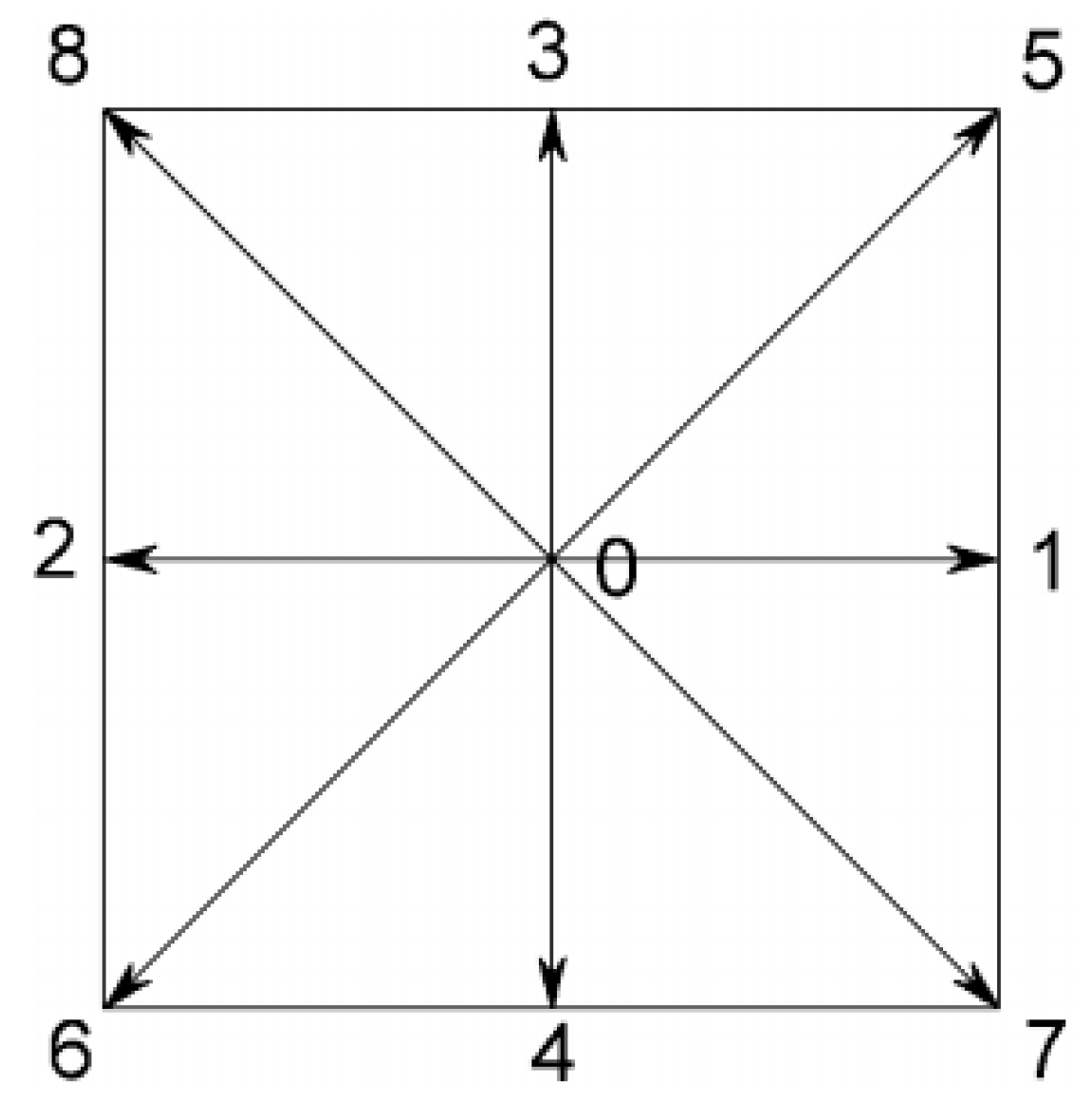
In this study, MRT-LBM is used to solve shallow water equations, and it has already been applied successfully by numerous researchers [6,29,31,32]. Our simulation is based on the $D_2{Q}_9$ model and space is discretized into a nine-speed square lattice (see Figure 1). The particle velocity $e_{\alpha }$ is defined as:

$$e_{\alpha }=\{\begin{array}{cc}0& \alpha =0,\\ \mathit{i}e\cos \left[\pi \left(\alpha -1\right)/2\right]+\mathit{j}e\sin \left[\pi \left(\alpha -1\right)/2\right]& \alpha =1-4\\ \sqrt{2}\mathit{i}e\cos \left[\pi \left(\alpha -1\right)/2+\pi /4\right]+\sqrt{2}\mathit{j}e\sin \left[\pi \left(\alpha -1\right)/2+\pi /4\right]& \alpha =5-8.\end{array},$$

(8)

The MRT-LBM contains two steps: a collision step and a streaming step:

$$\mathbf{Collision} \mathbf{and} \mathbf{Forcing} f_{\alpha }^{\prime }\left(\mathit{x},t\right)-f_{\alpha }\left(\mathit{x},t\right)=-{\mathit{M}}^{-1}\widehat{\mathit{S}}\left({\widehat{f}}_{\alpha }-{\widehat{f}}_{\alpha }^{eq}\right)+\frac{3\delta t{\omega }_{\alpha }}{e^2}{e}_{\alpha i}{F}_i,$$

(9)

$$\mathbf{Streaming} f_{\alpha }\left(\mathit{x},t+\delta t\right)=f_{\alpha }^{\prime }\left(\mathit{x}-e_{\alpha }\delta t,t\right) \alpha =0-8,$$

(10)

where $f_{\alpha }$ is the particle distribution function; the relationship between the distribution function and the moment is $\widehat{\mathit{f}}=\mathit{M}\mathit{f},\mathit{f}={\mathit{M}}^{-1}\widehat{\mathit{f}}$ and the bold-face symbols denote nine-dimensional column vectors, e.g., $\mathit{f}={\left[f_0,f_1,\cdots f_8\right]}^{\mathit{T}}$; ${\widehat{f}}_{\alpha }^{eq}$ is the equilibrium distribution functions of the moment ${\widehat{f}}_{\alpha }$; $f_{\alpha }^{\prime }$ is the post-collision state. Ginzburg [13] first proposed the general form of the transformation matrix $\mathit{M}$ which can be defined as [6,15,31]:

$$M=\left[\begin{array}{ccccccccc}1& 1& 1& 1& 1& 1& 1& 1& 1\\ -4& -1& -1& -1& -1& 2& 2& 2& 2\\ 4& -2& -2& -2& -2& 1& 1& 1& 1\\ 0& 1& 0& -1& 0& 1& -1& -1& 1\\ 0& -2& 0& 2& 0& 1& -1& -1& 1\\ 0& 0& 1& 0& -1& 1& 1& -1& -1\\ 0& 0& -2& 0& 2& 1& 1& -1& -1\\ 0& 1& -1& 1& -1& 0& 0& 0& 0\\ 0& 0& 0& 0& 0& 1& -1& 1& -1\end{array}\right].$$

(11)

$F_i$ is associated with the force term. In a $D_2{Q}_9$ model, the corresponding equilibrium distribution functions in the moment space ${\widehat{f}}_{\alpha }^{eq}$ are expressed as [6,15,31]:

$${\widehat{f}}_{\alpha }^{eq}=\{\begin{array}{ll}h,& \alpha =0,\\ 3g{h}^2/e^2-4h+3h(u_x^2+u_y^2)/e^2,& \alpha =1,\\ h{u}_y/e,& \alpha =2,\\ 4h-9g{h}^2/2e^2-3h\left(u_x^2+u_y^2\right)/e^2,& \alpha =3,\\ -h{u}_y/e,& \alpha =4,\\ h\left(u_x^2-u_y^2\right)/e^2,& \alpha =5,\\ -h{u}_x/e, & \alpha =6,\\ -h{u}_x/e,& \alpha =7,\\ h{u}_x{u}_y/e^2,& \alpha =8.\end{array}$$

(12)

$\widehat{\mathit{S}}$ is the relaxation matrix in the moment space:

$$\widehat{\mathit{S}}=\mathit{M}\mathit{S}{\mathit{M}}^{-1}=diag\left[s_1,s_2,s_3,s_4,s_5,s_6,s_7,s_8,s_9\right],$$

(13)

where $s_1=s_4=s_6=1$, $s_5=s_7=1.2$, $s_2=s_5-0.1$, $s_3=s_2-0.1$, $s_8=s_9=1/\tau$. With the eddy viscosity ${\nu }_e$ of the SGS model in consideration, $s_8$ and $s_9$ are decided as

$$s_8=s_9=\frac{1}{\tau +{\tau }_e}=\frac{1}{{\tau }_t},$$

(14)

where $\tau$ is the single relaxation time, ${\tau }_t$ is the total relaxation, and ${\tau }_e$ is the eddy relaxation time, which is given by [27,28]:

$${\tau }_e=\frac{-\tau +\sqrt{{\tau }^2+18C_s^2/\left(h{e}^2\right)\sqrt{{\prod }_{ij}{\prod }_{ij}}}}{2} ,$$

(15)

in which

$${\prod }_{ij}={\displaystyle \sum }_{\alpha }{e}_{\alpha i}{e}_{\alpha j}\left(f_{\alpha }-f_{\alpha }^{eq}\right).$$

(16)

$e_{\alpha i}$ is the velocity vector of a particle in the $i$ spatial coordinate.

In $\mathrm{LBM}$, the equilibrium distribution functions (EDFs) can be calculated by a Taylor series expansion of a Maxell–Boltzmann equilibrium distribution. According to constraint conditions of EDFs, the local equilibrium distribution $f_{\alpha }^{eq}$ for shallow water equations can be computed by the method of undefined coefficients [9,33], and $f_{\alpha }^{eq}$ can be expressed as:

$$f_{\alpha }^{eq}=\{\begin{array}{c}h-\frac{{\omega }_{\alpha }h}{e^2}\left(\frac{15}{8}gh+\frac{3}{2}{u}_j^2\right) \alpha =0,\\ \frac{{\omega }_{\alpha }h}{e^2}\left(\frac{3}{2}gh+3{\left(e_{\alpha }u\right)}_j+\frac{9}{2}{\left(e_{\alpha }u\right)}_j^2-\frac{3}{2}{u}_j^2\right) \alpha =1-8,\end{array}$$

(17)

where ${\omega }_{\alpha }$ is the weight coefficient, ${\omega }_0=4/9$, ${\omega }_{1-4}=1/9$, ${\omega }_{5-8}=1/36$.

The water depth $h$ and velocity$u$ can be calculated by the distribution function below:

$$h={\displaystyle \sum }_{\alpha =0}^8{f}_{\alpha },$$

(18)

$$u=\frac{1}{h}{\displaystyle \sum }_{\alpha =0}^8{e}_{\alpha }{f}_{\alpha }.$$

(19)

2.3. Curvilinear Coordinates

The lattice Boltzmann model on curvilinear coordinates was presented by using the GILBM [24].

The governing Equations (8) and (9) with orthogonal coordinates $\mathit{x}\equiv \left(x,y\right)$ are transformed into curvilinear coordinates $\mathsf{\epsilon }\equiv \left(\epsilon ,\eta \right)$, which can be written as

$$\mathbf{Collision} \mathbf{and} \mathbf{Forcing} f_{\alpha }^{\prime }\left(\mathbf{\epsilon },t\right)-f_{\alpha }\left(\mathbf{\epsilon },t\right)=-{\mathit{M}}^{-1}\widehat{\mathit{S}}\left({\widehat{f}}_{\alpha }-{\widehat{f}}_{\alpha }^{eq}\right)+\frac{3\delta t{\omega }_{\alpha }}{e^2}{e}_{\alpha i}{F}_i,$$

(20)

$$\mathbf{Streaming} f_{\alpha }\left(\mathbf{\epsilon },t+\delta t\right)=f_{\alpha }^{\prime }\left(\mathbf{\epsilon }-\Delta {\epsilon }_{\alpha },t\right) \alpha =0-8,$$

(21)

in which

$$\Delta {\epsilon }_{\alpha }={{\displaystyle \int }}_0^{\delta t}{\tilde{e}}_{\alpha }dt,$$

(22)

where ${\tilde{e}}_{\alpha }\equiv {\tilde{e}}_{\alpha ,i}$ is the particle velocity of curvilinear coordinates $\left(\epsilon ,\eta \right)$ and can be calculated as

$${\tilde{e}}_{\alpha ,i}=e_{\alpha ,j}\frac{\partial {\epsilon }_i}{\partial x_j}.$$

(23)

To calculate the contravariant velocities at each node, the estimation of the metrics is given by

$$\left[\begin{array}{cc}{\epsilon }_x& {\epsilon }_y\\ {\eta }_x& {\eta }_y\end{array}\right]=\frac{1}{J}\left[\begin{array}{cc}{y}_{\eta }& -x_{\eta }\\ -y_{\epsilon }& x_{\epsilon }\end{array}\right],$$

(24)

in which $J$ is described as

$$J=x_{\epsilon }{y}_{\eta }-x_{\eta }{y}_{\epsilon }.$$

(25)

To integrate the particle velocity, the second-order two-step Runge–Kutta method is used:

$$\mathrm{First} \mathrm{step}: \Delta {\epsilon }_{\alpha }{}^{\left(1\right)}=\frac{1}{2}\delta t{\tilde{e}}_{\alpha }\left(\epsilon \right);$$

(26)

$$\mathrm{Second} \mathrm{step}: \Delta {\epsilon }_{\alpha }=\delta t{\tilde{e}}_{\alpha }\left(\epsilon -\Delta {\epsilon }_{\alpha }{}^{\left(1\right)}\right)+o\left(\delta t^3\right).$$

(27)

The interpolation function is necessary to calculate the right-hand side of Equations (20) and (27). In both equations, the value between the grid points is required.

The second-order upwind quadratic interpolation is used, and can be expressed as

$${\mathrm{g}}_{\alpha }\left(\epsilon -\Delta {\epsilon }_{\alpha }\right)={\displaystyle \sum }_{m=0}^2{\displaystyle \sum }_{l=0}^2{a}_{\alpha ,m,2}{a}_{\alpha ,l,1}{\mathrm{g}}_{\alpha ,l,m},$$

(28)

where ${\mathrm{g}}_{\alpha ,l,m}$ is the stencil depending on the position of $\epsilon -\mathsf{\Delta }{\epsilon }_{\alpha }$. The coefficients are described as

$$\begin{array}{c}{a}_{\alpha ,0,i}=\frac{1}{2}\left(\left|\mathsf{\Delta }{\epsilon }_{\alpha ,i}\right|-1\right)\left(\left|\mathsf{\Delta }{\epsilon }_{\alpha ,i}\right|-2\right),\\ a_{\alpha ,1,i}=\left|\mathsf{\Delta }{\epsilon }_{\alpha ,i}\right|\left(\left|\mathsf{\Delta }{\epsilon }_{\alpha ,i}\right|-2\right),\\ a_{\alpha ,0,i}=\frac{1}{2}\left|\mathsf{\Delta }{\epsilon }_{\alpha ,i}\right|\left(\left|\mathsf{\Delta }{\epsilon }_{\alpha ,i}\right|-1\right).\end{array}$$

(29)

2.4. Boundary Conditions

Boundary conditions are significant and can affect the accuracy of the lattice Boltzmann method. The non-equilibrium extrapolation method [34] of second-order accuracy was chosen to determine the distribution functions at the boundaries from the given macroscopic variables:

$$f_{\alpha }\left({\mathbf{\epsilon }}_{\mathit{w}},t\right)=f_{\alpha }^{eq}\left(h_w,u_w\right)+f_{\alpha }^{\prime }\left({\epsilon }_f,t\right)-f_{\alpha }^{eq}\left(h_f,u_f\right),$$

(30)

where the subscript $w$ denotes the wall nodes and $f$ represents fluid nodes. The fluid water depth $h_f$ and macroscopic velocities $u_f$ can be computed from discharge or water level according to real cases.

For the wall nodes, since the water depth $h_w$ and the macroscopic velocities $u_w$ are not explicit, they are estimated from the neighboring fluid nodes. For the macroscopic velocities $u_w$, they can be estimated from the neighboring fluid velocities at the slip wall and are equal to zero at the non-slip wall. For the water depth, a three-point Lagrangian formula is applied [35]:

$$h_w={\displaystyle \sum }_{p=1}^3\left[h\left({\epsilon }_{f,p}\right){\displaystyle \prod }_{\mathrm{q}=1,\mathrm{q}\ne \mathrm{p}}^3\frac{{\epsilon }_w-{\epsilon }_{f,q}}{{\epsilon }_{f,p}-{\epsilon }_{f,q}}\right].$$

(31)

In our simulation, the criterion of steady states is defined as

$$\frac{{\mathsf{\Sigma }}_{ij}\left|u_{ij}^{n+1}-u_{ij}^n\right|}{{\mathsf{\Sigma }}_{ij}\left|u_{ij}^{n+1}\right|}\le 1.0\times {10}^{-7}.$$

(32)

3. Model Simulation and Discussion

In this part, an open channel flow with a 180° bend is investigated to test the accuracy of the proposed scheme. Moreover, a real meandering river with piers is simulated to test the application of the coupled model. The results of the simulation and a discussion are presented as follows.

3.1. Open Channel Flow with a 180° Bend

De Vriend [36] experimentally studied the 180° open channel, and it has also been used by many researchers to validate their models [26,37,38]. Zhang [38] has established a 3D Re-Normalisation Group (RNG) $\mathrm{k}-\mathsf{\epsilon }$ turbulence model with curvilinear coordinates to simulate meandering rivers and channels. Therefore, it is appropriate to compare these results with ours. The studied channel is 1.7 m wide and the centerline radius is $\mathrm{R}=4.25 \mathrm{m}$. There are two 6-m long straight reaches connected to the bend. The channel boundaries are hydraulically smooth and the bed slop is zero. The upstream flow discharge is 0.19 m³/s and the downstream value is given with the terminal water depth ${\mathrm{H}}_0=0.18 \mathrm{m}$. A uniform mesh of $100\times 26$ (Figure 2) with $\delta x=\delta y=0.047 \mathrm{m}$ is employed, the particle velocity $e$ is 2 m/s, and the Froude number $\mathrm{Fr}=0.47$. Also, the chosen time step is $\delta t=\delta x/e=0.0235 \mathrm{s}$ and the relaxation time is $\mathsf{\tau }=0.819 \mathrm{s}$, as determined by Equation (3).

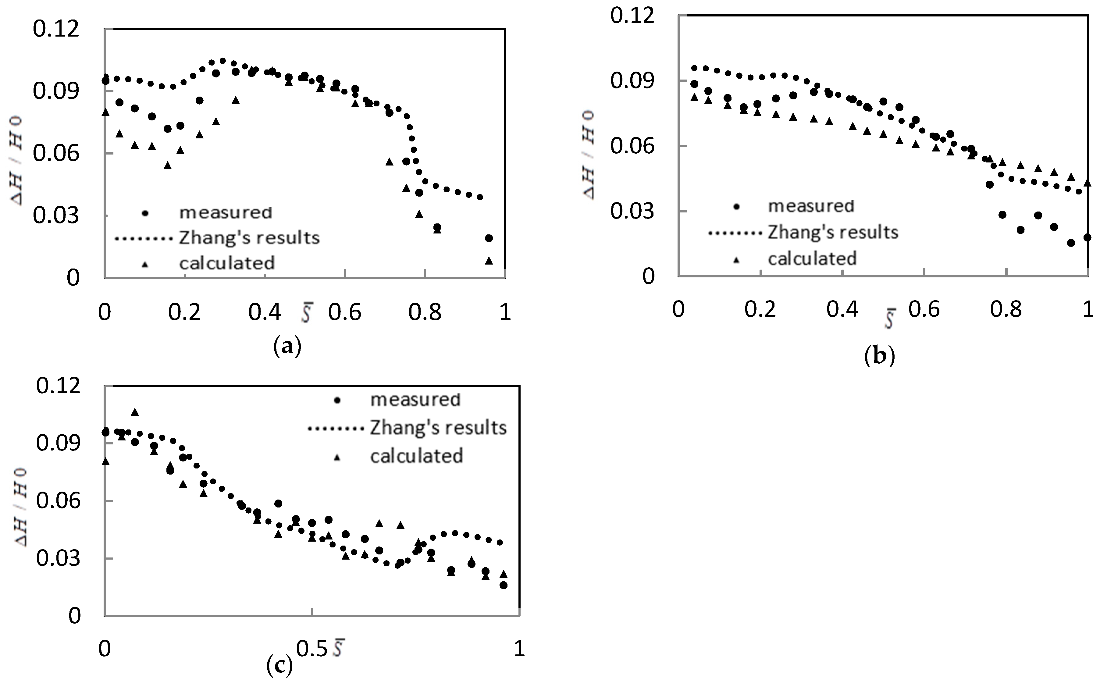
Comparison of the water depth at the central line as well as the inner and outer banks are depicted in Figure 3. The error analysis of different models is presented in

Table 1. Error analysis of water depth simulation.

Model	Inner Bank			Center Line			Outer Bank
	MAE	RMSE	RRE (%)	MAE	RMSE	RRE (%)	MAE	RMSE	RRE (%)
2D-LBM	0.0094	0.011	14.1	0.0085	0.011	15.7	0.011	0.013	16.7
3D	0.0077	0.0099	12.5	0.0096	0.012	16.5	0.0089	0.012	14.5

(1) MAE is mean absolute error; RMSE is root mean squared error, which is the average of the squared differences between measured and predicted values; RRE is defined as the ratio of the RMS error to the observed change. (2) The unit of MAE and RMSE is m. (3) The three-dimensional (3D) model is a 3D Re-Normalisation Group (RNG) k-ε turbulence model established by Zhang [38].

. For LBM, the maximum root mean squared error(RMSE) and the relative RMS error (RRE), which occurred at the outer bank, are 0.013% and 16.7%, respectively. In Zhang’s 3D model, these values are 0.012% and 16.5%, which occurred at the center line. Simulations at the inner bank for the two models are better than that at the central line and the outer bank, since the relative RMS error at the inner bank is the smallest. In general, compared to the experimental data, our 2D scheme achieved an acceptable result in the water depth, but a closer agreement between the experimental data and results of the 3D model was realized.

Comparisons between predicted and measured depth-averaged velocities at six cross-sections are depicted in Figure 4; the error analyses of different sections are shown in

Table 2. Error analysis of velocities at different sections.

Model	$0°$		$30°$		$60°$		$90°$		$120°$		$180°$
	MAE	RMSE	MAE	RMSE	MAE	RMSE	MAE	RMSE	MAE	RMSE	MAE	RMSE
2D-LBM	0.0185	0.023	0.052	0.061	0.037	0.044	0.062	0.063	0.076	0.08	0.013	0.017
3D	0.0180	0.021	0.027	0.028	0.056	0.063	0.049	0.058	0.035	0.04	0.056	0.06

Note: (1) The unit of MAE and RMSE is m/s. (2) The 3D model is a 3D RNG k-ε turbulence model established by Zhang [38].

. At section 60° and 180°, our scheme achieved better results and the RMS error values were 0.06 and 0.017, while in the remaining sections the 3D model performed better. For both methods, the maximum RRS error occurred at section 90° and the values were 0.063 and 0.058 (see Table 2). Generally, although there are some discrepancies at section 90°, the comparison of results between the measured data and predicted data was acceptable.

The results of water depth and velocities indicate that Zhang’s model achieved better results. The main reason for this is that Zhang’s model is established as a 3D RNG k-ε turbulence model, which considers the vertical direction and the influence of the secondary flow in the meandering channel. Nevertheless, as our scheme is a 2D model, it is simpler in programming and the results show reasonable accuracy.

3.2. Meandering River with Piers

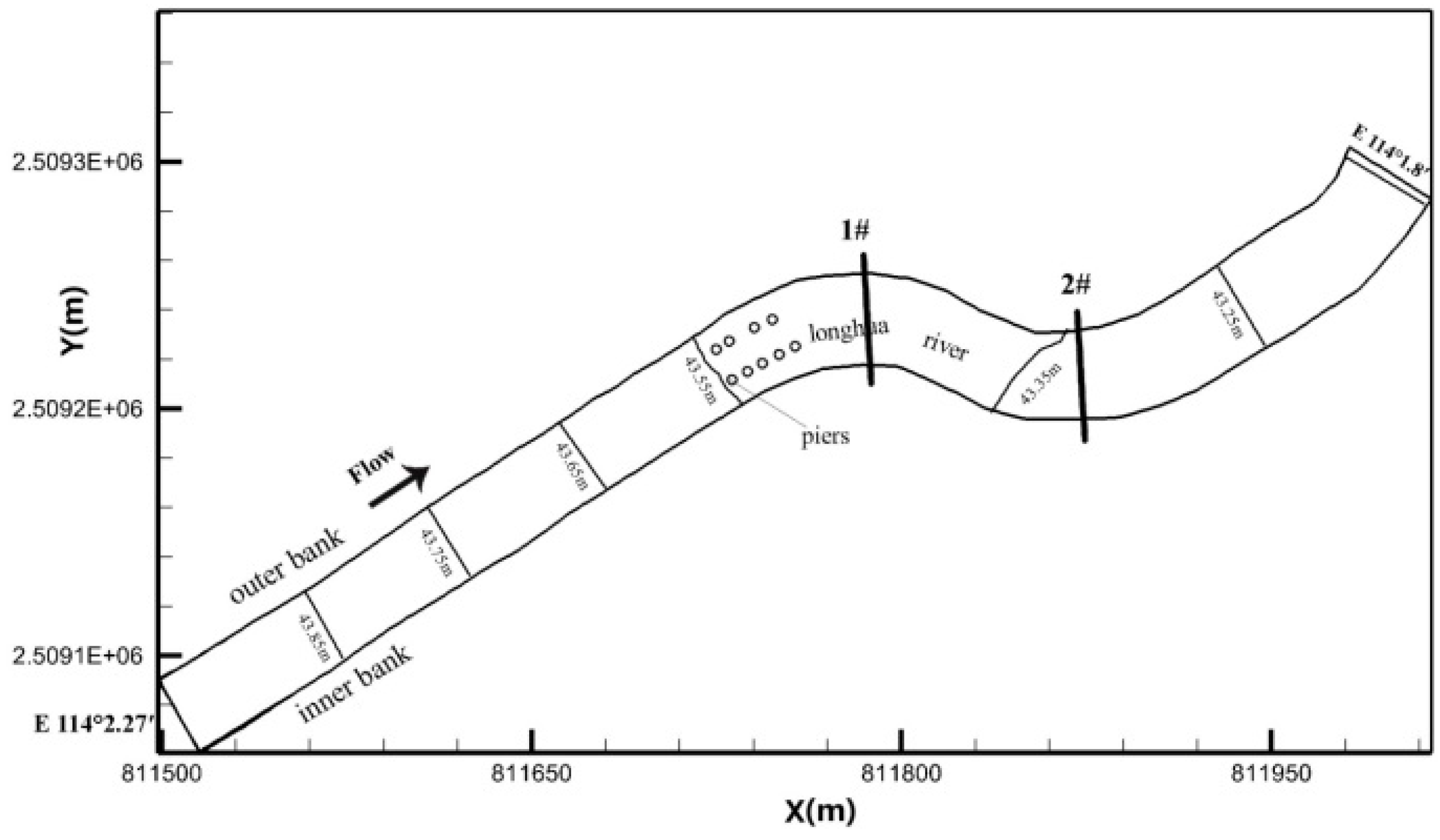
In order to test the capability of simulating the practical problem in real rivers, the present scheme was used to simulate the meandering flow of the Longhua River in Shenzhen, China. This study area is 606 m long and 31.5 m wide with two bend sections (section 1$\#$ and section 2$\#$). Figure 5 shows a schematic description of the simulation domain. White circles depicted in the figure represent the piers in this river, across which there is a small bridge.

The accuracy and stability of the traditional finite volume method (FVM) has been demonstrated in the simulation of practical rivers [39,40]. Therefore, our results were compared with FVM results and monitoring data. The monitoring data were obtained by monitoring the river on 8 August 2017, for which water depth and depth-average velocities were monitored at the bends. There were four monitoring points set every 10 m from the inner bank at each bend.

The main parameters are described in

Table 3. Parameters for the simulation.

Method	Grid	$Q$ (m/s)	${\mathit{H}}_0$ (m)	Bed Slope	${\mathit{n}}_{\mathit{b}}$	E (m/s)	$\mathsf{\delta }t$	$\mathsf{\tau }$	Re
MRT-LBM	316 × 20	494	5.22	0.00373	0.025	10	0.05	0.5001	156.83
FVM	5934	494	5.22	0.00373	0.025	/	0.05	/	156.83

Notes: Triangle meshes are used in FVM, therefore it shows different meshes. This river is an artificial river, so that the bed slope is constant. $R_e=156.83$ is the Reynolds number, which can be defined as: $R_e=h{U}_0/2\upsilon$, where $h$ is the height of the entry section, $\upsilon$ is the kinematic viscosity, and $U_0$ is the maximum inlet velocity.

. The upstream discharge was 494 m³/s and the downstream water depth was 5.22 m. The Manning’s coefficient of the bed $n_b$ was 0.025 and constant particle velocity was $\mathrm{e}=10 \mathrm{m}/\mathrm{s}$. The time step was $\delta t=0.05 \mathrm{s}$ and the single relaxation time was $\mathsf{\tau }=0.56 \mathrm{s}$.

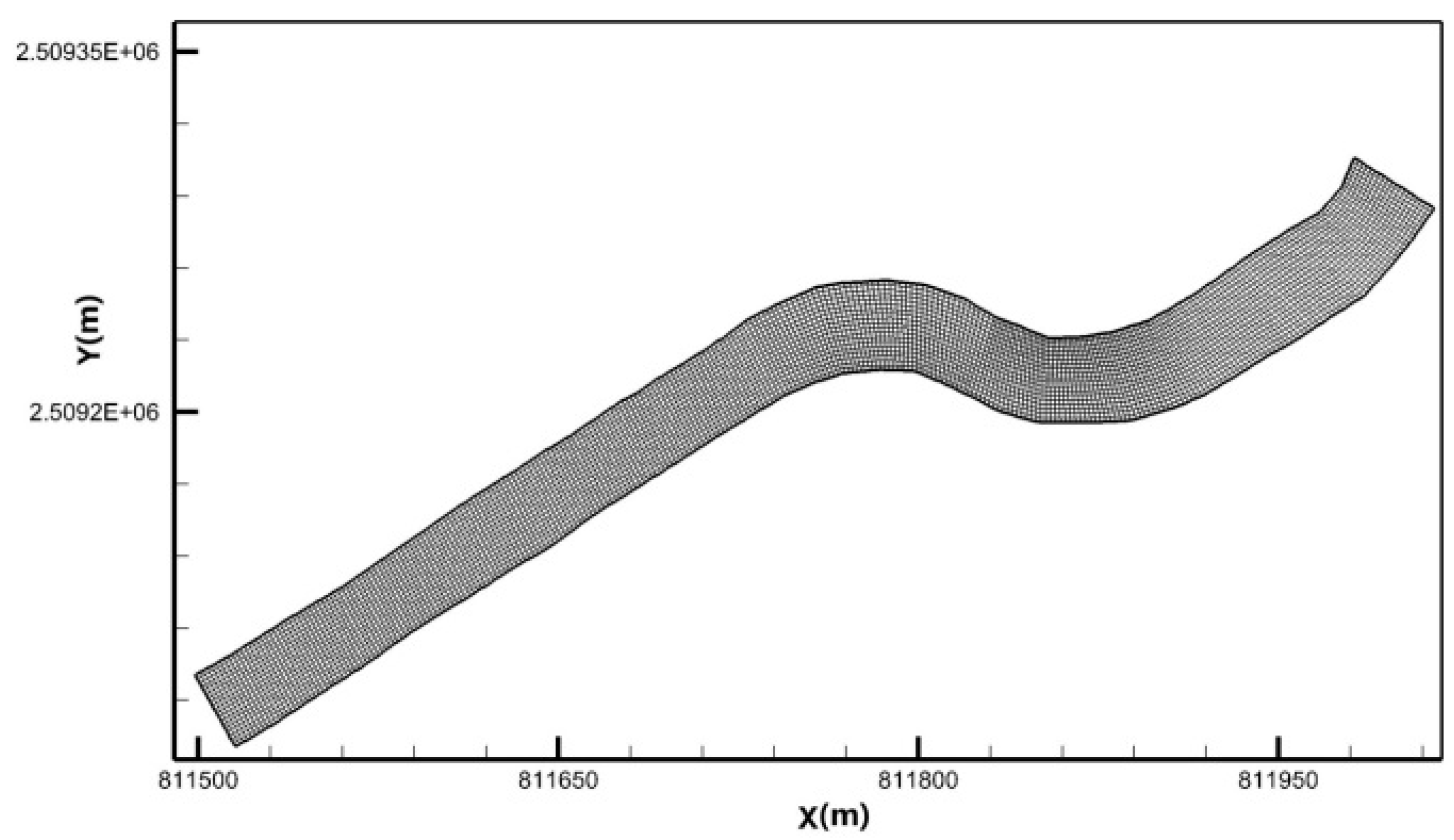
In LBM simulations, body-fitted coordinate grids were used and a uniform mesh of 316 × 20 (see Figure 6) was applied. The minimum lattice length was 1.00035 m, while the diameter of piers was 1.2 m. Like the wall boundaries, these piers were simulated as obstacles, and a slip boundary transformed on curvilinear coordinates was used.

In the FVM model, the Reynolds-averaged Navier–Stokes equations (RANS) were solved to simulate piers, and triangle meshes were used. The minimum element area was 0.66 m².

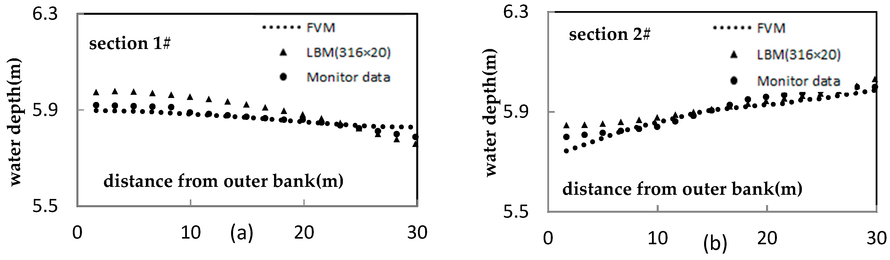
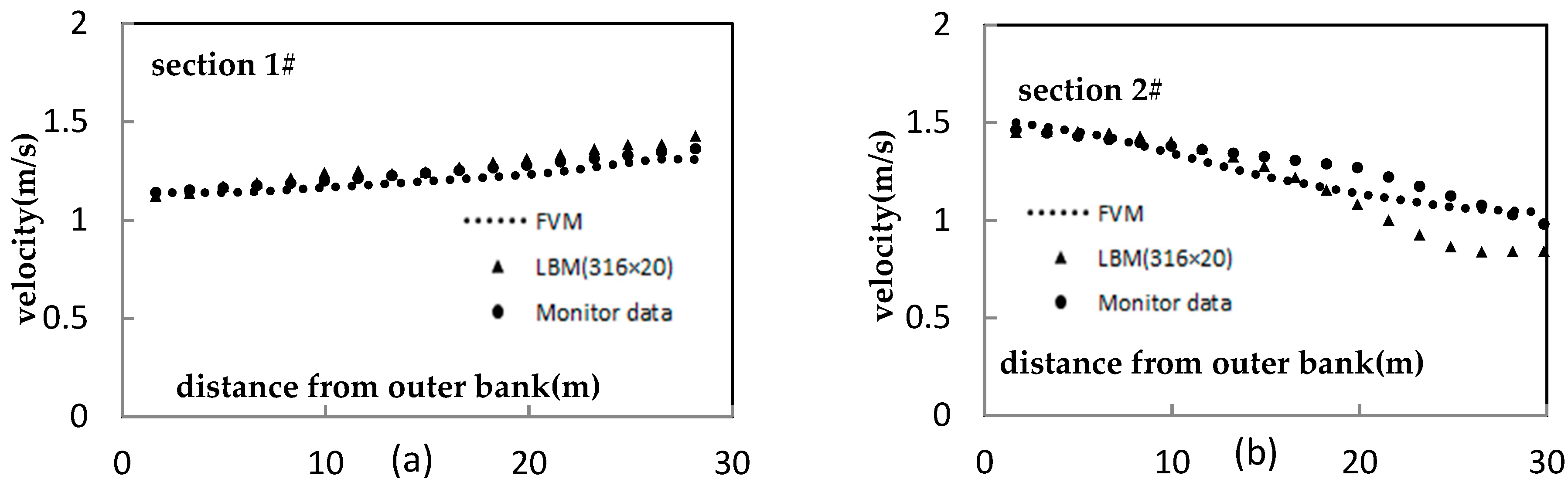
A comparison was made at the bends of the river. The water depth at the bends are plotted in Figure 7, and the total velocity is shown in Figure 8. The water depth of section 1# decreases from the outer bank to the inner bank, while at section 2# the water depth decreases from the inner bank to the outer bank. The total velocity shows a decreasing trend from the inner bank to the outer bank in section 1#, while in the bend section 2# displays an increasing trend from the inner bank to the outer bank. This outcome is consistent with the actual situation; where the water depth is higher, the water flows more slowly.

Table 4. Error analysis of the simulation model.

Variables	Model	Section 1#			Section 2#
		MAE	RMSE	RRE (%)	MAE	RMSE	RRE (%)
Water depth	MRT-LBM	0.018	0.020	15.1	0.022	0.026	13.0
	FVM	0.014	0.018	13.7	0.021	0.025	12.5
Velocity	MRT-LBM	0.033	0.039	16.4	0.106	0.14	29.1
	FVM	0.039	0.042	17.5	0.061	0.07	15.1

shows the error analysis of the FVM and the MRT-LBM. Both methods agree well. For example, the water depth in the FVM achieves a better result, as the RMSE is 0.025 m and the relative RMS error is 12.5% at section 2#, while for MRT-LBM the RRE is 13.0% and the RMSE is 0.026 m. Generally, there are minute differences between monitored data and simulation data‒–this is probably due to the influence of centrifugal force which generates the secondary flow at the bend, while the 2D computation model does not consider the vertical direction. However, the accuracy is acceptable.

According to the comparison, our scheme performs well for velocity at section 1#, while at section 2# there are some discrepancies near from the inner bank and the RRE is 29.1%. In general, the FVM was superior to the proposed model. The main reason for this are: (1) the uniform mesh of the MRT-LBM is non-orthogonal, which may lead to small deviation especially at bends; (2) the governing equations should be transformed into curvilinear coordinates in the proposed model, and the finite difference approximation of the transformation matrix may lead to some discrepancies. However, our proposed model requires much fewer CPUs as well as less time for simulation. The outcome demonstrates the advantages of LBM and is consistent with relevant reports in the literature [12,15,41].

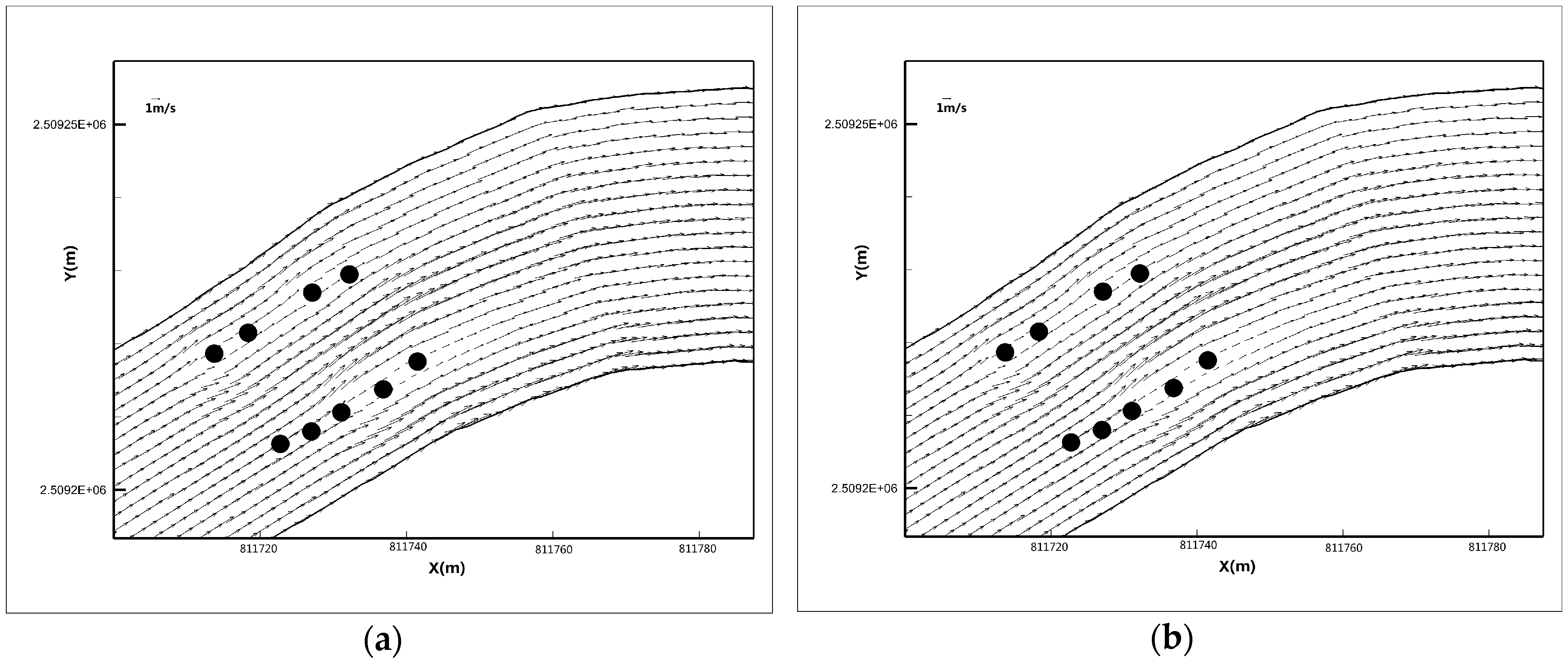
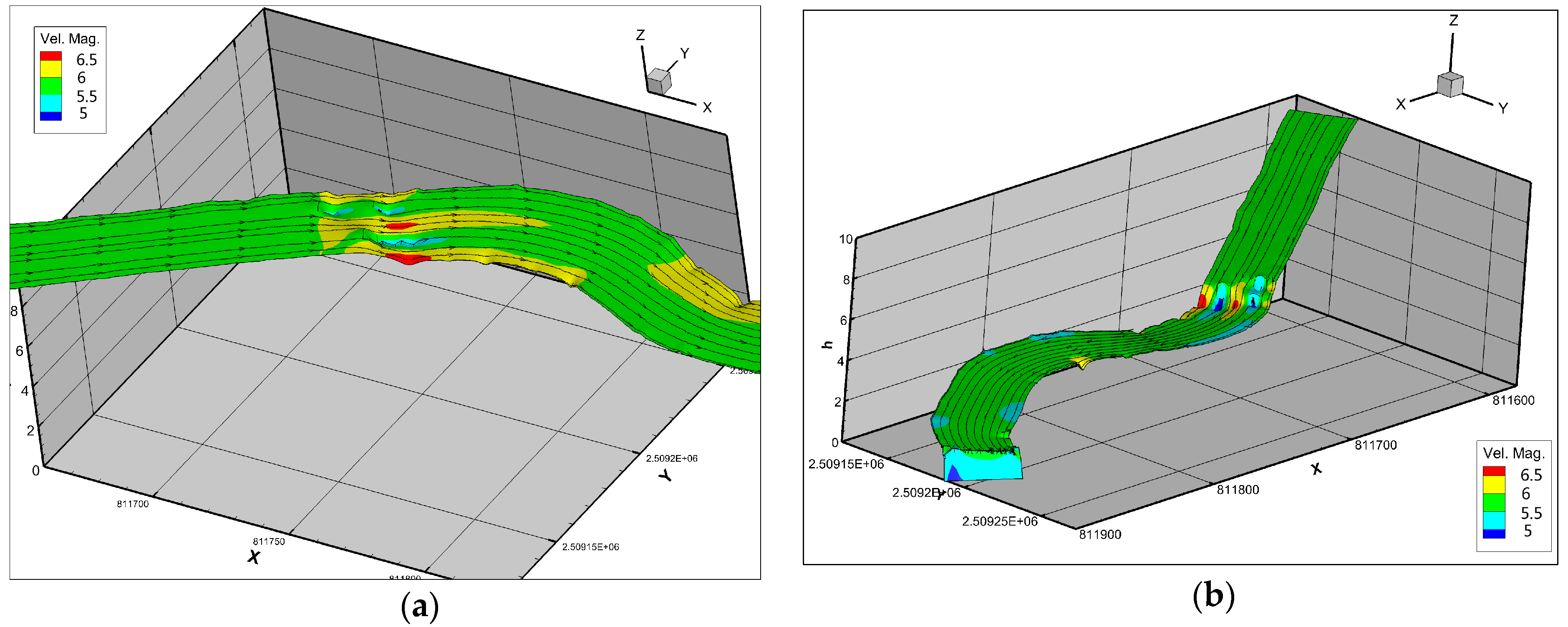
Two uniform meshes of 316 × 20 and 632 × 40 (see Figure 6) were applied to investigate the flow field distribution around the piers. The results in Figure 9 show that the finer grids produce a more clear flow field around the cylinders. Figure 10 depicts a 3D visualization of the streamline and water depth, which shows small vortexes around the piers. Because of the low Reynolds number, the water flows past the piers and persists without separation.

4. Conclusions

In this study, a sub-grid multiple relaxation time (MRT) lattice Boltzmann model with curvilinear coordinates was developed. An open channel flow with a $180°$ bend was simulated to validate the model. Furthermore, the calculated results were compared with the experimental data and Zhang’s results. Error analysis revealed that the 3D model was superior to the proposed 2D model; however, the 2D model only requires simple programming and its results are acceptable.

A real meandering river with piers was simulated to test the application of the scheme. The results were reliable and agreed well with those of the finite volume method (FVM). Flow field and 3D streamline with height are plotted in Figure 9 and Figure 10, in which the flow around the piers can be clearly seen. It was shown that with a low Reynolds number, the proposed method has great potential to solve realistic problems in curved rivers.

In the future, turbulent models with a high Reynolds number can be modified based on the proposed method to solve more complex flow problems. Moreover, the advection and anisotropic dispersion equations can be combined to solve the water quality problems. These extensions will be studied in our future research.

References

- Rivet, J.P.; Boon, J.P. Lattice Gas Hydrodynamics; Cambridge University Press: London, UK, 2001; pp. 204–210. [Google Scholar]
- Rothman, D.H.; Zaleski, S.; Adam, I.V. Lattice-gas cellular automata: Simple models of complex hydrodynamics. Comput. Phys. 1998, 12, 576. [Google Scholar] [CrossRef]
- Qian, Y.H.; d’Humières, D.; Lallemand, P. Lattice bgk models for Navier-Stokes equation. Europhys. Lett. 1992, 17, 479. [Google Scholar] [CrossRef]
- Chen, S.Y.; Doolen, G. Lattice Boltzmann method for fiuid fiows. Annu. Rev. Fluid Mech. 1998, 30, 329–364. [Google Scholar] [CrossRef]
- Zhao, Z.M.; Huang, P.; Li, Y.N.; Li, J.M. A Lattice Boltzmann method for viscous free surface waves in two dimensions. Int. J. Numer. Methods Fluids 2013, 71, 223–248. [Google Scholar] [CrossRef]
- Li, Y.N.; Huang, P. A coupled Lattice Boltzmann model for advection and anisotropic dispersion problem in shallow water. Adv. Water Res. 2008, 31, 1719–1730. [Google Scholar] [CrossRef]
- Shan, X.; Doolen, G. Multi-component Lattice-Boltzmann model with interparticle interaction. J. Stat. Phys. 1995, 81, 379–393. [Google Scholar] [CrossRef]
- Luo, L.S. Theory of the Lattice Boltzmann method: Lattice Boltzmann models for nonideal gases. Phys. Rev. E 2000, 62, 4982–4996. [Google Scholar] [CrossRef]
- Salmon, R. The Lattice Boltzmann method as a basis for ocean circulation modeling. J. Mar. Res. 1999, 57, 503–535. [Google Scholar] [CrossRef]
- Guo, Z.J. A Lattice Boltzmann model for the shallow water equations. Comput. Methods Appl. Mech. Eng. 2002, 191, 3527–3539. [Google Scholar]
- Tubbs, K.R.; Tsai, F.T.C. Multilayer shallow water flow using Lattice Boltzmann method with high performance computing. Adv. Water Res. 2009, 32, 1767–1776. [Google Scholar] [CrossRef]
- Luo, L.S.; Liao, W.; Chen, X.; Peng, Y.; Zhang, W. Numerics of the Lattice Boltzmann method: Effects of collision models on the Lattice Boltzmann simulations. Phys. Rev. E Stat. Nonlinear Soft Matter Phys. 2011, 83, 1–24. [Google Scholar] [CrossRef] [PubMed]
- Ginzburg, I. Equilibrium-type and link-type Lattice Boltzmann models for generic advection and anisotropic-dispersion equation. Adv. Water Res. 2005, 28, 1171–1195. [Google Scholar] [CrossRef]
- Ginzburg, I. Generic boundary conditions for Lattice Boltzmann models and their application to advection and anisotropic dispersion equations. Adv. Water Res. 2005, 28, 1196–1216. [Google Scholar] [CrossRef]
- Lallemand, P.; Luo, L.S. Theory of the Lattice Boltzmann method: Dispersion, dissipation, isotropy, galilean invariance, and stability. Phys. Rev. E 2000, 61, 6546–6562. [Google Scholar] [CrossRef]
- He, X.Y.; Luo, L.S.; Dembo, M. Some progress in Lattice Boltzmann method. Part I. Nonuniform mesh grids. J. Comput. Phys. 1996, 129, 357–363. [Google Scholar] [CrossRef]
- Filippova, O.; Hänel, D. Grid refinement for lattice-bgk models. J. Comput. Phys. 1998, 147, 219–228. [Google Scholar] [CrossRef]
- Crouse, B.; Rank, E. A lb-based approach for adaptive flow simulations. Int. J. Mod. Phys. B 2003, 17, 109–112. [Google Scholar] [CrossRef]
- Yu, D.Z.; Mei, R.W.; Wei, S. A multi-block Lattice Boltzmann method for viscous fluid flows. Int. J. Numer. Methods Fluids 2002, 39, 99–120. [Google Scholar] [CrossRef]
- Neumann, P.; Bungartz, H.-J. Dynamically adaptive Lattice Boltzmann simulation of shallow water flows with the peano framework. Appl. Math. Comput. 2015, 267, 795–804. [Google Scholar] [CrossRef]
- Budinski, L. Mrt lattice boltzmann method for 2d flows in curvilinear coordinates. Comput. Fluids 2014, 96, 288–301. [Google Scholar] [CrossRef]
- He, X.Y.; Luo, L.S.; Dembo, M. Some progress in the Lattice Boltzmann method_reynolds number enhancement in simulations. Physica A 1997, 239, 276–285. [Google Scholar] [CrossRef]
- Shyam Sunder, C.; Babu, G.B.V.; Strenski, D. Parallel performance of the interpolation supplemented lattice boltzmann method. Lect. Notes Comput. Sci. 2003, 2913, 428–437. [Google Scholar]
- Imamura, T.; Suzuki, K.; Nakamura, T.; Yoshida, M. Acceleration of steady-state Lattice Boltzmann simulations on non-uniform mesh using local time step method. J. Comput. Phys. 2005, 202, 645–663. [Google Scholar] [CrossRef]
- Qu, K.U.N.; Shu, C.; Chew, Y.T. An isoparametric transformation-based interpolation-supplemented Lattice Boltzmann method and its application. Mod. Phys. Lett. B 2010, 24, 1315–1318. [Google Scholar] [CrossRef]
- Zhao, Z.M.; Huang, P.; Li, S.T. Lattice Boltzmann model for shallow water in curvilinear coordinate grid. J. Hydrodyn. B 2017, 29, 251–260. [Google Scholar] [CrossRef]
- Hou, S.L.; Sterling, J.; Chen, S.Y.; Doolen, G. A Lattice Boltzmann subgrid model for high reynolds number flows. Fields Inst. Commun. 1996, 6, 151–166. [Google Scholar]
- Zhou, J.G. A Lattice Boltzmann model for the shallow water equations with turbulence modeling. Int. J. Mod. Phys. C 2002, 13, 1135–1150. [Google Scholar] [CrossRef]
- Yu, H.; Luo, L.-S.; Girimaji, S.S. Les of turbulent square jet flow using an mrt Lattice Boltzmann model. Comput. Fluids 2006, 35, 957–965. [Google Scholar] [CrossRef]
- Smagorinsky, J. General circulation experiments with the primitive equations, I. The basic experiment. Mon. Weather Rev. 1963, 91, 99–152. [Google Scholar] [CrossRef]
- Peng, Y.; Zhou, J.G.; Burrows, R. Modelling solute transport in shallow water with the Lattice Boltzmann method. Comput. Fluids 2011, 50, 181–188. [Google Scholar] [CrossRef]
- Peng, Y.; Zhou, J.G.; Zhang, J.M.; Liu, H. Lattice Boltzmann modeling of shallow water flows over discontinuous beds. Int. J. Numer. Methods Fluids 2014, 75, 608–619. [Google Scholar] [CrossRef]
- Dellar, P.J. Nonhydrodynamic modes and a priori construction of shallow water Lattice Boltzmann equations. Phys. Rev. E 2002, 65, 036309. [Google Scholar] [CrossRef] [PubMed]
- Guo, Z.L.; Zheng, C.G.; Shi, B.C. Non-equilibrium extrapolation method for velocity and pressure boundary conditions in the Lattice Boltzmann method. Chin. Phys. 2002, 11, 366–374. [Google Scholar]
- Hay, D.R.; Mechlih, H. Control of systems partially unknown variable structure approach. Am. Control Conf. 1994, 1, 1174–1175. [Google Scholar]
- Vriend, H.J.D. A mathematical model of steady flow in curved shallow channels. J. Hydraul. Res. 1976, 15, 37–54. [Google Scholar] [CrossRef]
- Ye, J.; McCorquodale, J.A.; Barron, R.M. A three-dimensional hydrodynamic model in curvilinear coordinates with collocated grid. Int. J. Numer. Methods Fluids 1998, 28, 1109–1134. [Google Scholar] [CrossRef]
- Zhang, M.L.; Shen, Y.M. Three-dimensional simulation of meandering river based on 3-d rng κ-ɛ turbulence model. J. Hydrodyn. B 2008, 20, 448–455. [Google Scholar] [CrossRef]
- LeVeque, R.J. Balancing source terms and flux gradients in high-resolution godunov methods: The quasi-steady wave-propagation algorithm. J. Comput. Phys. 1998, 146, 346–365. [Google Scholar] [CrossRef]
- Bermudez, A.; Vazquez, M.E. Upwind methods for hyperbolic conservation laws with source terms. Comput. Fluids 1994, 23, 1049–1071. [Google Scholar] [CrossRef]
- Noble, D.R.; Georgiadis, J.G.; Buckius, R.O. Comparison of accuracy and performance for lattice boltzmann and finite difference simulations of steady viscous flow. Int. J. Numer. Methods Fluids 1996, 23, 1–18. [Google Scholar] [CrossRef]
Figure 1.
Discrete lattice of the model.
Figure 2.
Computational mesh of the open channel bend.
Figure 3.
Comparison of water depth along the channel: (a) outer bank; (b) central line; (c) inner bank. Note: The vertical ordinate is the water depth which is normalized as . The horizontal axis represents the longitudinal length from the inlet, which is normalized against the distance at the center of the bend.
Figure 4.
Velocity distribution of different sections (a) 0°; (b) 30°; (c) 60°; (d) 90°; (e) 120°; (f) 180°.
Figure 5.
Schematic description of the simulation domain.
Figure 6.
Mesh of the lattice Boltzmann method (316 × 20).
Figure 7.
Comparison of water depth: (a) comparison results of section 1#; (b) comparison results of section 2#. The horizontal axis represents the distance from the outer bank, and the unit is m.
Figure 8.
Comparison of depth average velocity: (a) comparison results of section 1#; (b) comparison results of section 2#. The horizontal axis represents the distance from the outer bank, and the unit is m.
Figure 9.
Flow field around the piers: (a) uniform mesh of 316 × 20; (b) uniform mesh of 632 × 40. The black dots represent the piers.
Figure 10.
3D visualization of water depth and streamline in different perspectives: (a) the back view; (b) the front view.