Indirect Damage of Urban Flooding: Investigation of Flood-Induced Traffic Congestion Using Dynamic Modeling
by

Jingxuan Zhu
1, 
Qiang Dai
1,2,3,*,
Yinghui Deng
1,
Aorui Zhang
1,
Yingzhe Zhang
1 and
Shuliang Zhang
1,3,* 1
Key Laboratory of VGE of Ministry of Education, Nanjing Normal University, Nanjing 210023, China
2
Water and Environmental Management Research Centre, Department of Civil Engineering, University of Bristol, Bristol BS8 1TR, UK
3
Jiangsu Center for Collaborative Innovation in Geographical Information Resource Development and Application, Nanjing 210023, China
*
Authors to whom correspondence should be addressed.
Water 2018, 10(5), 622; https://doi.org/10.3390/w10050622
Submission received: 17 March 2018
/
Revised: 5 May 2018
/
Accepted: 7 May 2018
/
Published: 10 May 2018
(This article belongs to the Section Urban Water Management)
Abstract
:In many countries, industrialization has led to rapid urbanization. Increased frequency of urban flooding is one consequence of the expansion of urban areas which can seriously affect the productivity and livelihoods of urban residents. Therefore, it is of vital importance to study the effects of rainfall and urban flooding on traffic congestion and driver behavior. In this study, a comprehensive method to analyze the influence of urban flooding on traffic congestion was developed. First, a flood simulation was conducted to predict the spatiotemporal distribution of flooding based on Storm Water Management Model (SWMM) and TELAMAC-2D. Second, an agent-based model (ABM) was used to simulate driver behavior during a period of urban flooding, and a car-following model was established. Finally, in order to study the mechanisms behind how urban flooding affects traffic congestion, the impact of flooding on urban traffic was investigated based on a case study of the urban area of Lishui, China, covering an area of 4.4 km2. It was found that for most events, two-hour rainfall has a certain impact on traffic congestion over a five-hour period, with the greatest impact during the hour following the cessation of the rain. Furthermore, the effects of rainfall with 10- and 20-year return periods were found to be similar and small, whereas the effects with a 50-year return period were obvious. Based on a combined analysis of hydrology and transportation, the proposed methods and conclusions could help to reduce traffic congestion during flood seasons, to facilitate early warning and risk management of urban flooding, and to assist users in making informed decisions regarding travel.
1. Introduction
Urbanization is the process of concentrating population, resources, and wealth. It stimulates the development of economic globalization and plays an important role in promoting the economic growth of developing countries. However, opportunity and risk coexist in relation to urbanization. Both the risk of, and exposure to, hazards increase rapidly in urban areas because of the concentration of population and wealth, exhaustion of resources, and changes in environmental conditions and human activities. Urban flooding, which is one of the problems exacerbated by urbanization, has a direct impact on traffic flow and indirect effects on production and the livelihoods of the urban population.
The study of the impact of urban flooding on traffic congestion using dynamic modeling mainly includes traffic simulation and flood simulation. Traffic models can be divided into three categories: macroscopic, microscopic, and mesoscopic [1]. At the macro level, Greenshields [2] described the connection between lane density and speed with his fundamental diagram. Sugihakim and Alatas [3] investigated traffic flow on a road network when considering different road conditions. Manley et al. [4] elucidated that traffic dynamics are the product of behaviors and interactions of individuals. Micro traffic models studied traffic phenomena by taking each individual vehicle as a starting point and analyzing its interactions with other vehicles [5]. The most popular microscopic traffic model is the car-following model [6,7], which is part of an agent-based model (ABM) [8]. Many models are devoted to solving the problem of traffic congestion. For example, Ben-Akiva et al. [9] dynamically simulated traffic congestion using elastic arrival rates during peak periods.
Urban flooding occurs when rainfall runoff exceeds sewer capacity, resulting in surface flow accumulating on the road surface without entering the sewer. Generally, there are two main types of drainage systems: minor and major. Djordjević et al. [10] proposed the dual-drainage concept, stressing the importance of considering the interaction between the two systems. Major drainage systems include the surface flood channels, while minor systems comprise the drainage sewer network. Depending on their characteristics, major systems can be modeled by either one-dimensional (1D) or two-dimensional (2D) models, while minor systems are often modeled using a 1D model. Leandro [11] categorized the existing models into two classes: research-based applications and commercial software packages. Compared with the 1D/1D model MIKE FLOOD [12], the 1D/2D model MIKE FLOOD and MIKE 21 [13] provided better fits to time series data, according to Carr and Smith [14]. Chen et al. [15] simulated the complex flow process on an overland surface of pluvial flooding cases using two research-based applications, i.e., SIPSON and UIM. Spry and Zhang [16] modeled two distinct case studies using the 1D/1D models XP-SWMM and DRAINS. TELEMAC-2D is also an efficient open-source hydrodynamic model, which was developed initially by the National Hydraulics and Environment Laboratory of the Research and Development Directorate of the French Electricity Board [17].
Many studies have investigated the impact of rainfall on traffic flow using traffic and flood simulations. For example, Cools et al. [18] found that rainfall diminishes traffic intensity (i.e., the number of cars passing along a specific segment of road). Lin and Nixon [19] considered the effects of adverse weather on traffic crashes based on a systematic review and meta-analysis. Their results indicated that the crash rate usually increases during periods of precipitation. Urban road traffic dynamics are the product of the behaviors and interactions of thousands or often millions of individuals [4], and rainfall affects the behavioral decisions of drivers. Goodwin [20] concluded that weather affects traffic flow by reducing visibility, decreasing pavement friction, and impairing driver behavior and vehicle performance. Billot et al. [21] focused on the impact of rain on driver behavior, and they revealed that drivers tend to reduce speed and increase both headway and spacing during periods of rainfall. Su et al. [22] proposed an integrated simulation method for flood and traffic congestion under urban rainstorms based on the Storm Water Management Model (SWMM) for flood simulation and the results of a questionnaire survey for modeling human behavior. These previous studies have clearly elucidated the influence of rainfall on traffic flow and driver behavior. However, despite flooding being more likely than rainfall to cause traffic congestion and to result in continuous impact on traffic flow, few studies have considered its importance.
The aims of this study were to develop a method using the SWMM–TELEMAC2D integrated model (a combination of TELEMAC-2D and SWMM by exchanging information at the connecting nodes; Section 2.2) and an ABM (Section 2.3) to simulate flood-induced traffic congestion under varying conditions and implement it in a real city for a pilot study. Several specific scenarios were considered including diverse rainfall return periods and various durations of flood occurrence. Additionally, in order to improve the microscopic traffic analysis, the dynamic features of the real world were considered. This method was applied to a case study of an actual urban area. As traffic simulation can be a useful tool for traffic control systems, the results of the study will be beneficial. For policy makers in assessing the appropriateness of local road and traffic arrangements and implementing strategic improvements.
2. Study Area and Models
2.1. Study Area
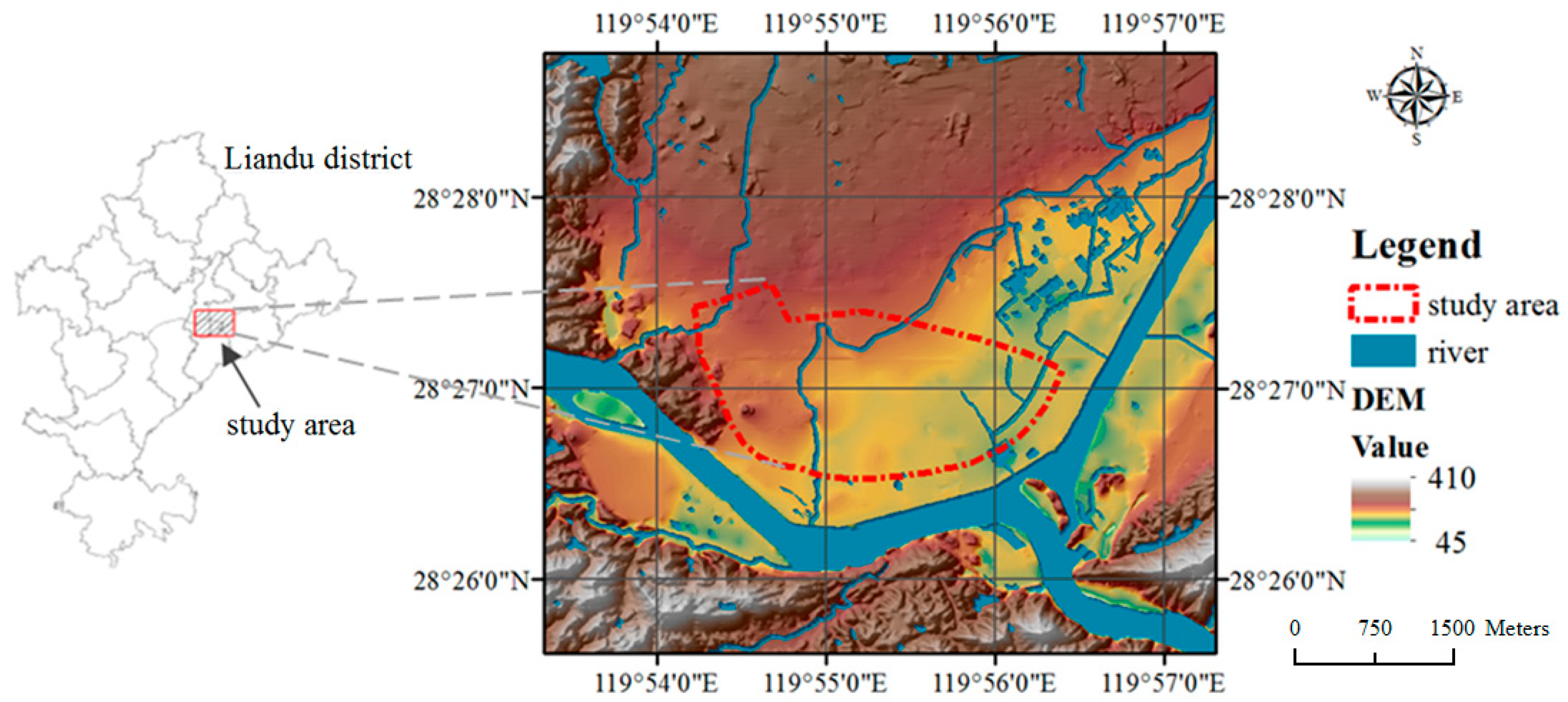
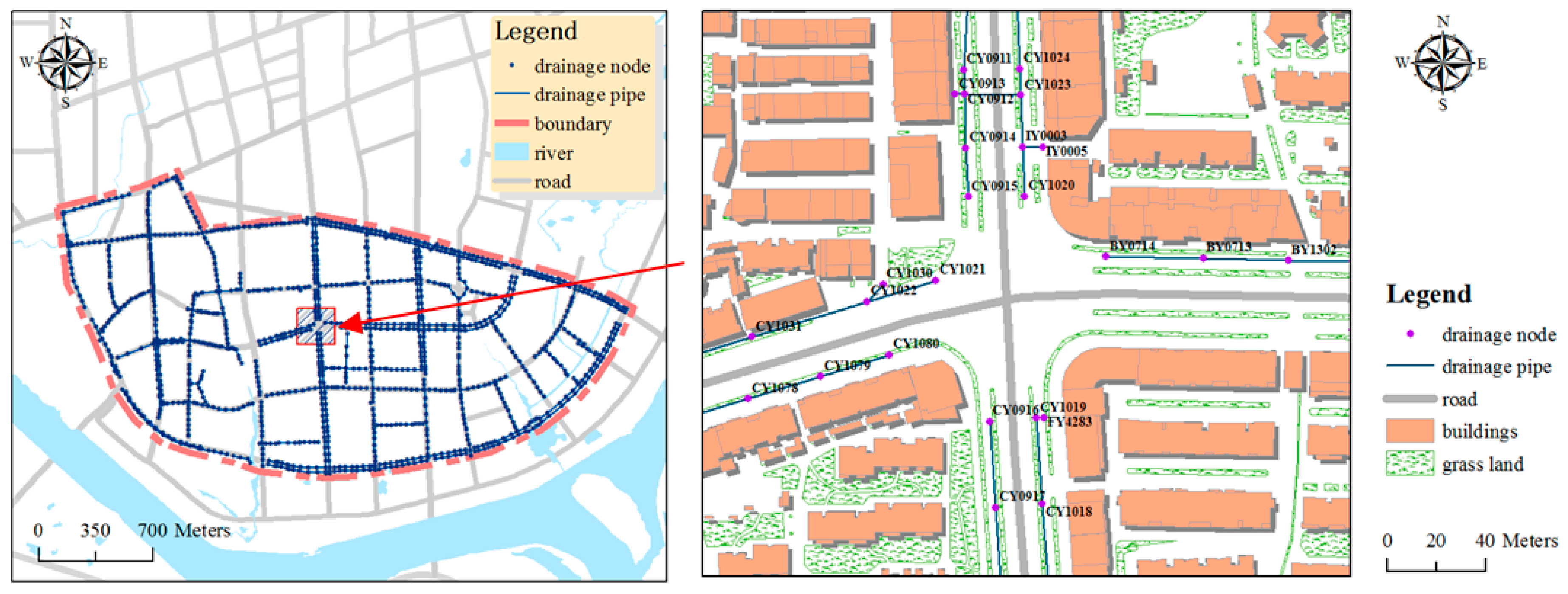
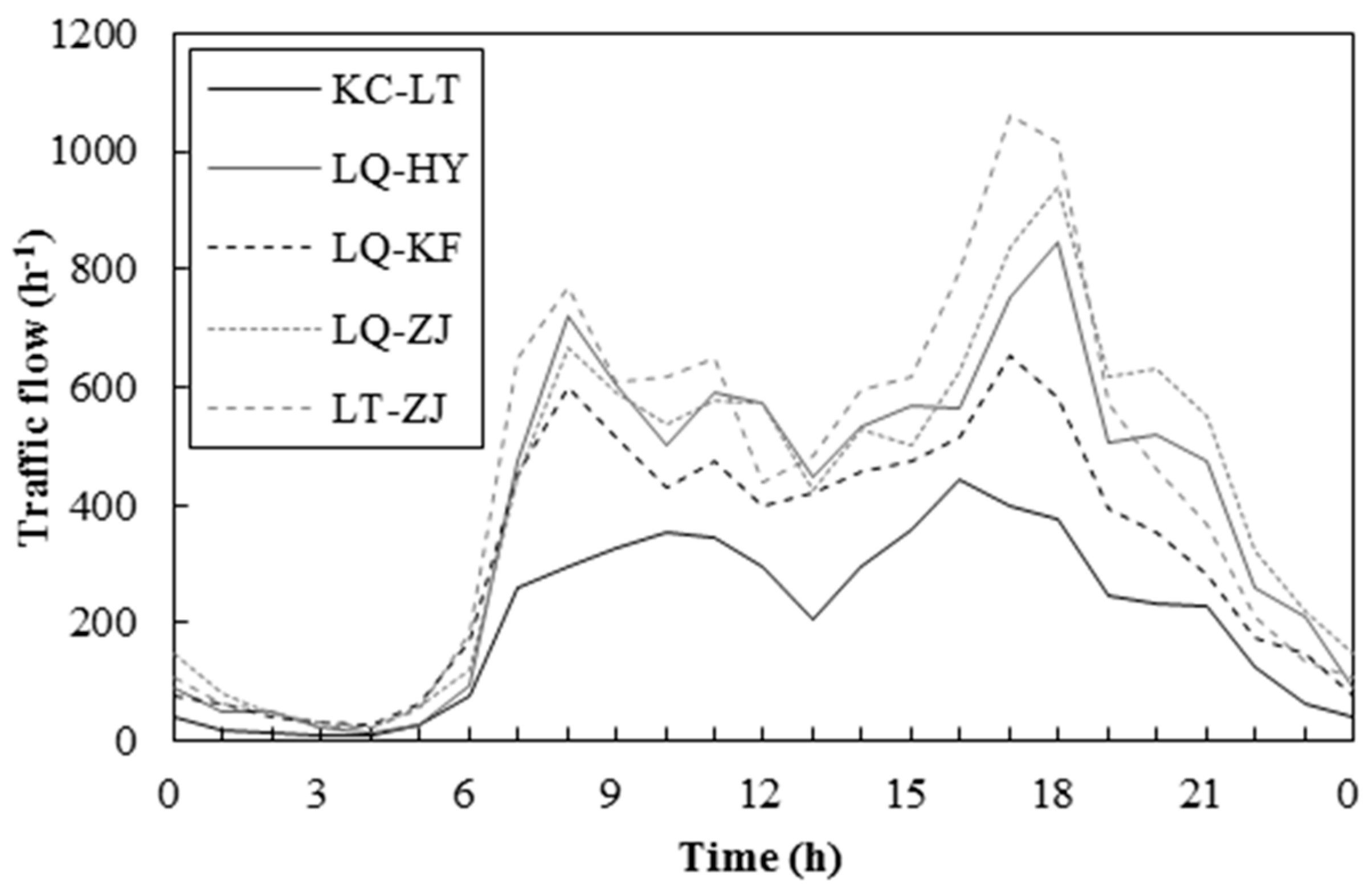
The city of Lishui in Zhejiang Province was considered as the experimental region in this study. The urban district of Lishui is mainly a hilly and mountainous area, with a river named Oujiang running across its southern and eastern parts. Because of the subtropical monsoon climate, Lishui is hot and rainy in summer. During the Meiyu flood period in May and June, the frequencies of heavy rainstorms and persistent concentrated rainfall events both rise sharply. The city can also be affected by typhoons in midsummer, which often result in flooding-related disasters. On 20 August 2014, a heavy rainfall event lasting a few days produced a 50-year flood in Lishui, causing considerable loss of property. The traffic system was also seriously affected and the main roads were completely flooded. The study area mainly covers the central district of Lishui with an area of 4.4 km2 and has a large population and intensive traffic flow (see Figure 1). Because the influence of rainfall on lower grade roads is not obvious, we selected nine main roads for this study: Li Yang Street (LY), Li Qing Street (LQ), Jie Fang Street (JF), Kai Fa Road (KF), Lu Tang Street (LT), Dong Gang Road (DG), Kuo Cang Road (KC), Hua Yuan Road (HY), and Zi Jin Road (ZJ). As preparation, we compiled basic geographic data (Figure 2), drainage network data (Figure 3), and annual rainfall data. We also obtained accurate traffic flow data (traffic flow in this paper refers to the number of vehicles passing through a node within one hour) at five intersections from 24 June 2017 to 7 July 2017 in this area, along with rainfall data. Figure 4 shows an example of the traffic flow data acquired on one day (3 July 2017).
2.2. SWMM–TELEMAC2D Integrated Model
In order to simulate flooding in a realistic manner, sewer network models must be coupled with overland flow models [23]. Generally, a 1D model is used for calculating the rainfall–runoff hydrographs and flow conditions in drainage networks, while a 2D model is employed for routing flow on an overland surface [24]. We chose a 1D dynamic sewer network model (SWMM) for the simulation of the sewer network (minor system). The network system was formed by a set of links and nodes, and the flow traveled through the links from node to node. For the ground surface system, we applied the TELEMAC-2D model.
SWMM is a dynamic urban flood simulation program used primarily for single events or long-term (continuous) simulations of runoff and water quality in urban areas. With SWMM, a drainage system can be generalized as a series of water and material flows between several major environmental components. It is used widely for planning, analysis, and design related to storm water runoff in urban areas [25].
In the SWMM model, the Horton scheme was used for infiltration. Dynamic Wave routing and ponding-allowed schemes were chosen in this study. This means that the excess volume will flow into the ponded area evenly so that errors will increase as the ponded area enlarges. Thus, the TELEMAC-2D model will be used for further adjustment, and the stored volumes simulated by SWMM will enter the 2D model as a source. TELEMAC-2D solves depth-averaged free surface flow equations, as derived first by Barré de Saint-Venant in 1871. The main results produced for each node of the computational mesh are the water depth and the depth-averaged velocity components [17]. This hydrodynamic model solves the equations of non-structured grids with triangular (or quadrilateral) finite elements. The nature of the finite element mesh allows for the fitting of elements of various sizes within a specified boundary, which allows high resolution in areas of increased bed slope or narrow channels and low resolution in areas where detail is not required [26].
The difficulty of hydrologic simulation lies in the spatial discretization (see Section 3.1) and setting of parameters. Generally, flood modeling requires the preparation of four sets of data. The first dataset comprises hydrologic data, especially local historical rainfall data or simulated rainfall data designed by formulas. The second dataset includes drainage network data, e.g., the lengths and diameters of the underground drainage pipes within the study area and the depths of rainwater wells. The third dataset consists of the details of the underlying surface, such as the slope and impermeability of each subcatchment, which determine the surface runoff process. The fourth dataset defines the boundary attributes of the outlet nodes that connect to storage units or rivers.
Generally, the interaction of discharge and the synchronization of timing are the two main steps in linking a 2D overland flow model with a 1D sewer network model [15,23,24]. Discharge is based on the water level at the surface (h2d), hydraulic head at the manhole (h1d), and ground surface elevation (Z2d). Drainage is determined by the following equations; when h1d < Z2d, a weir equation is used (Equation (1)), and, when h1d > Z2d, an orifice equation is selected (Equation (2)):
where Q is the interacting discharge (m3/s), cw is the weir discharge coefficient, w is the weir crest width (m), Amh is the manhole area (m2), and c0 is the orifice discharge coefficient.
The TELEMAC-2D model step subroutine is used to synchronize the two models. This is a necessary procedure because of the difference in the time steps between both models [15,23]. We consider the SWMM run time as the synchronization time (Tsync). In this way, the TELEMAC-2D model time step is adjusted whenever its run time is expected to exceed the synchronization:
In this study, the water exchange between two models is achieved using the following approach. In the location of manhole, if h1d > Z2d, the excess volume in the urban drainage system (modeled by SWMM) will flow into the ground surface (modeled by TELEMAC-2D). After that, when h1d < Z2d, surface water will enter the urban drainage system from the surface again.
2.3. Agent-Based Model
An ABM is a type of computational model that can simulate the actions and interactions of autonomous agents in order to assess their effects on the system. An ABM has the ability to incorporate both spatially and temporally explicit data, model bidirectional relations between individual human agents and the macroscale behavior of the social or environmental system, capture emerging patterns at higher scales of the system that result from interactions at lower levels, and blend qualitative and quantitative approaches [27].
This type of model has a wide range of applications in various fields. During recent decades, ABMs have gained popularity in the analysis of complex traffic systems. When applied to traffic simulations, although each vehicle follows specific rules, the aggregate behavior of all vehicles can be represented by a specific probability distribution function. In an agent-based traffic simulation model, both space and time are considered discrete. Therefore, it is possible to observe the parameters of the behavior of each individual vehicle as well as their interactions with other vehicles. It also provides the possibility to experiment with many alternatives and to derive results in real time [3]. In order to simulate the effect of urban flooding on traffic, the urban flood model is firstly driven to obtain continuous changes of water depth under different situations, and the traffic-simulated model identifies these changes and generates the corresponding responses for the traffic. This approach can improve the performance in modeling the agents’ behavior in response to the combination of flood models and an ABM.
3. Methodology
Our research comprised three aspects: environmental simulation, behavioral study, and comprehensive analysis. The first of these steps included traffic and flooding simulations based on geographic information system (GIS) data and flood data simulated by SWMM. Analysis of the observations and actions of drivers constituted the behavioral study. Finally, the developed model was combined with the results of the previous two steps to estimate flood-induced traffic congestion under different scenarios due to the uncertainty of the events.
3.1. Environmental Simulation of Traffic and Flooding
Traffic systems are complex and diverse because of their complicated rules and variety of network configurations. A robust traffic model should include details of the traffic environment (e.g., roads, junctions, and traffic lights), operating rules, and individual vehicles. In this study, we used NetLogo for the traffic simulation. As an agent-based programmable modeling environment, NetLogo provides a platform with which modelers can disseminate instructions to hundreds or thousands of “agents” [28].
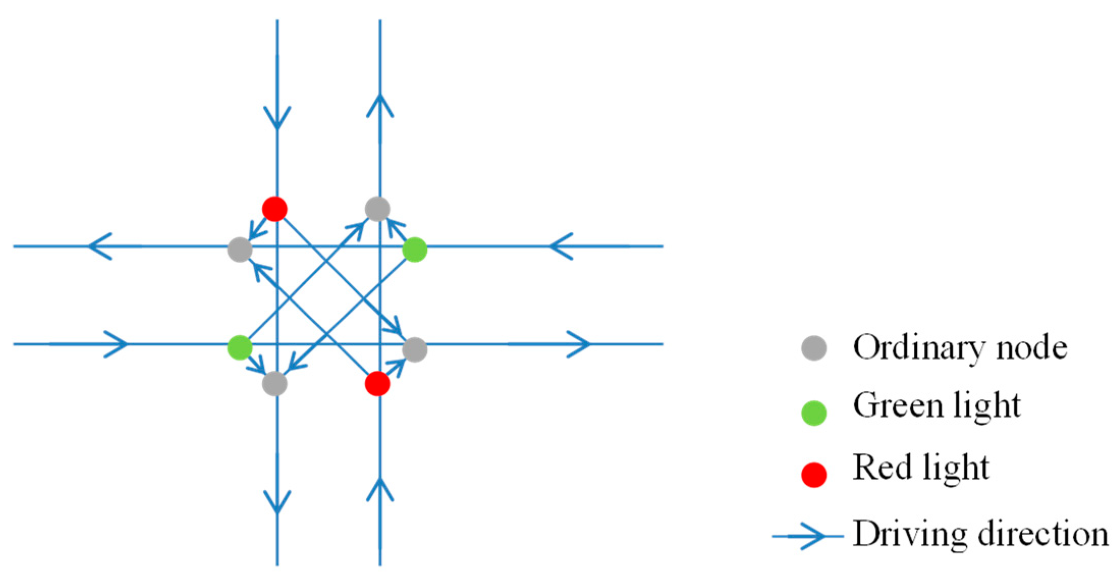
In our study, traffic was modeled using a 1D model. One way in which a surface network can be discretized (in a 1D model) is to consider the domain as a set of nodes connected by links [29]. Here, the nodes represent traffic junctions, and the links are roads. The modeled structure at a crossroad junction is shown in Figure 5. There are three cases for the traffic lights at the junction. First, only the lights of the west and east directions are green. Second, only the lights of the north and south directions are green. Finally, all the lights are red. The traffic lights were changed according to actual conditions.
The flood situation was another necessary element of the environment in this study. Generally, rainfall affects traffic in two respects: flood depth and visibility. As visibility is difficult to describe and simulate, flood depth was taken as the focus of our research. The process to obtain the flood depth comprised three components: subcatchment discretization, rainfall data acquisition, and runoff simulation. The point of the first step was to ensure that each subcatchment was connected to only one orifice.
We used GIS Engine components to discretize the study area automatically, and the regional watersheds were extracted using the digital elevation model data and GIS hydrologic analysis methods. The subcatchments were produced based on geographic information with different sizes and shapes, with special consideration given to the influence of buildings and roads on the water movement. This formed the basis for the subsequent analysis. The method ensured that all surface runoff in a subcatchment would rush into the drainage network through the junction node before ultimately flowing into the river via the outlet node.
The simulated rainfall was analyzed to obtain the rainfall intensity of different regression periods using the equations presented in Section 3.3. The changes in continuous surface runoff were obtained for the various hydrologic processes using different time-varying rainfall events simulated by the two flood models. The results of water depth for each of the subcatchments were reported every five minutes.
3.2. Agent Behavior in Regular Driving Pattern
The study of agent behavior constituted a main feature of this research. In the simulation, when the leading vehicle changes speed, it sets off a chain reaction among other vehicles, which is called “car-following”. Additionally, each of the drivers has their own specific destination in the system. It is assumed that each driver will choose the “best” direction at each junction. A series of such behaviors was simulated to analyze their impact on traffic congestion.
The study of relationships between vehicles is fundamental in traffic congestion research, especially in terms of the characteristics of vehicles following one another on a roadway. Many car-following theories have been established, including follow-the-leader models [30], the Gazis–Herman–Rothery model [31], and safety distance or collision avoidance models [32]. Krauß [33] introduced a car-following model based on the recognition that vehicles generally move without colliding into one another. We established the model at discrete time steps t = t + 1 based on the Nagel–Schreckenberg cellular automata (CA) model of vehicular traffic on highways [34], because the method of the CA model is more similar to an ABM. The steps adopted were as follows:
where xn and vn denote the position and speed of the n-th vehicle, respectively, vmax is the speed limit, a is the maximum acceleration of the vehicle, d is a parameter that can adjust the maximum achievable speed calculated by the first two steps, and Δx is the distance between the leading and following vehicles, i.e., Δx = xn+1 − xn. Here, v represents the distance that a vehicle will move during a time step (units in meters); v and x have the same units, so they can be seen as parallel in these equation. The relationship between a and v is similar.
In this CA model, the above four steps are repeated in order at each time step, and all vehicles are updated in parallel. The acceleration step directs vehicles to move as rapidly as possible (within the maximum speed limit). Step 2 checks the speed to avoid collisions between two adjacent vehicles. The randomization step is important, because it ensures the model is not a deterministic algorithm, which exactly reflects the unique concept of ABM. The speed of the n-th vehicle is decreased randomly with probability p if vn > 0. It considers the different behaviors of individual drivers when slowing down, which contribute to the development of traffic congestion. Finally, all vehicles move based on the number of cells equal to their v value.
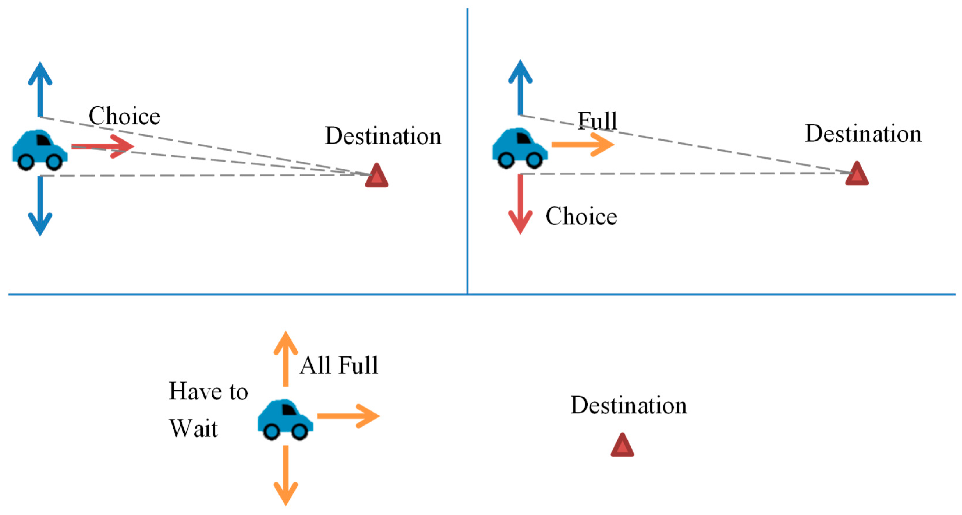
The main motivation of the traffic model implemented in this study was the destination of each driver. Before arriving at a junction, a driver chooses the direction they will follow next. In most cases, drivers choose the direction that takes them closer to their destination based on perceptual experience. However, if the desired road is already completely full, the driver has to make a decision: choose the next most preferred road or wait at the junction if no other options are available. In reality, the choice of direction is not absolute because of uncertainty, which means it is difficult to simulate accurately. Therefore, to simplify the model, our study ignored this problem. Figure 6 shows the three conditions regarding direction selection at a junction.
Road congestion is a condition that occurs as use increases, and is characterized by slower speeds, longer trip times, and increased vehicular queuing. When traffic demand is great enough that the interaction between vehicles slows the speed of the traffic stream, it results in considerable congestion [35]. In this study, we used the road crowding degree to indicate road congestion:
where Ce is the road capacity, L is the length of the road, N is the number of lanes, l is the average vehicle length, Pe relates to the degree of road congestion, and n is the actual number of vehicles on the road.
In the implemented ABM, each driver has their own identity, perception, and characteristics including age, gender, level of education, and spirit of adventure. Among them, spirit of adventure is assigned randomly, meaning that a small range of random additions and subtractions are made on the mean value. For example, women have a lower tolerance for flooding, so they have a lower speed than men in the same water depth. Other attributes also have the same effects on driver behavior in the traffic flow. However, it is difficult to measure the driver’s behaviors through strictly physical ways. Data collected by questionnaires is an efficient method and can effectively reflect people’s response to emergencies. When a flood occurs, drivers adjust their speed based on their perception of the water depth. The results obtained by Su et al. [22], who used a questionnaire to establish driver behavior under conditions of flooding and low visibility in rain, are considered accurate. In our study, the socioeconomic data from the Land and Statistical Bureau (such as income, education, etc.) and questionnaires are both used to determine the parameters of ABM (see Table 1).
3.3. Scenario Design
The time of occurrence, location, and intensity of a rainstorm or flood cause different impacts on road traffic. In order to increase the accuracy and fidelity of our simulation, we defined two types of scenarios: time of flood occurrence and rainfall intensity. The former was divided into two cases (worst and best). The worst case reflected the occurrence of a rainstorm/flood event during rush hour, while the best case considered the occurrence of the event during a leisure period. These two cases could be switched easily by changing the number of vehicles running on the road. In this study, the traffic flow of a road was determined based on the number of vehicles at the entrance. By observing traffic flow data, we analyzed the traffic conditions in the study area. We selected 12 start times for the storm at 2-h intervals beginning at 00:00. The reason for choosing 2-h rainfall periods in the simulation was that the Chicago hyetograph is recognized as one of the most suitable ways for simulating heavy rainfall during a 2-h period in China [36]. If the duration of the simulated rainfall lasted over two hours, the error would increase. Therefore, this period was adopted for convenience of later comparison between different scenarios. In addition, traffic volume is affected by many factors (such as local weather, policies, festivals, and people’s preferences), which have daily, weekly, and seasonal cycles. The quantitative analysis of the possible uncertainties associated with the traffic simulation will be investigated in future work. For example, it is impossible to know accurate traffic flow data for the following day. All the parameters in our model were adjustable to simulate the various conditions, e.g., the traffic volume at each entrance and the proportion exiting at vehicles’ destinations. Table 2 presents the parameter variations used in the simulation scenarios.
The scenario considering rainfall intensity was based on the rainfall return period, e.g., 5 years, 20 years, and so on. Heavy rainstorms have long return periods, while light rain events have short return periods. As rainfall intensity is related closely to the return period, we used the storm intensity equation to simulate rainfall of different intensities.
We simulated a rainfall series with an accuracy of one minute using the Chicago hyetograph based on the storm intensity formula. The results of the simulation were considered appropriate for rainfall simulating and suitable for comparison between different situations.
Rainfall intensity relates to the average rainfall of a continuous rainfall period, which can be calculated using the following formula:
where i is the rainfall intensity (mm/min), t is the duration of the rainfall event (min), and h is the total rainfall (mm).
Assuming that rainfall is distributed evenly within the catchment area, we selected the maximum rainfall intensity of the rain event as the design basis. The storm intensity equation was then derived based on local rainfall records for many years:
where q is the rainfall intensity (L/s · 104 m2), p is the rainfall recurrence period (year), t is the duration of the rainfall event (min), and A1, c, b, and n are local parameters.
The traffic flow and rainfall data, as well as the water depth data calculated based on the different rainfall intensities used in the flood model, were input into NetLogo to simulate agent behavior and produce traffic congestion at different times. We obtained depth distribution maps from the integrated flood model at five-minute intervals, where depth is reflected by the grid color. Then, we imported it into NetLogo as a basis for the drivers to simulate the depth of the water in front of them. The average value of the crowding degree was obtained from repeated simulations (100 times in this work) of the traffic for each scenario.
4. Results
4.1. Results of Flooding Simulation
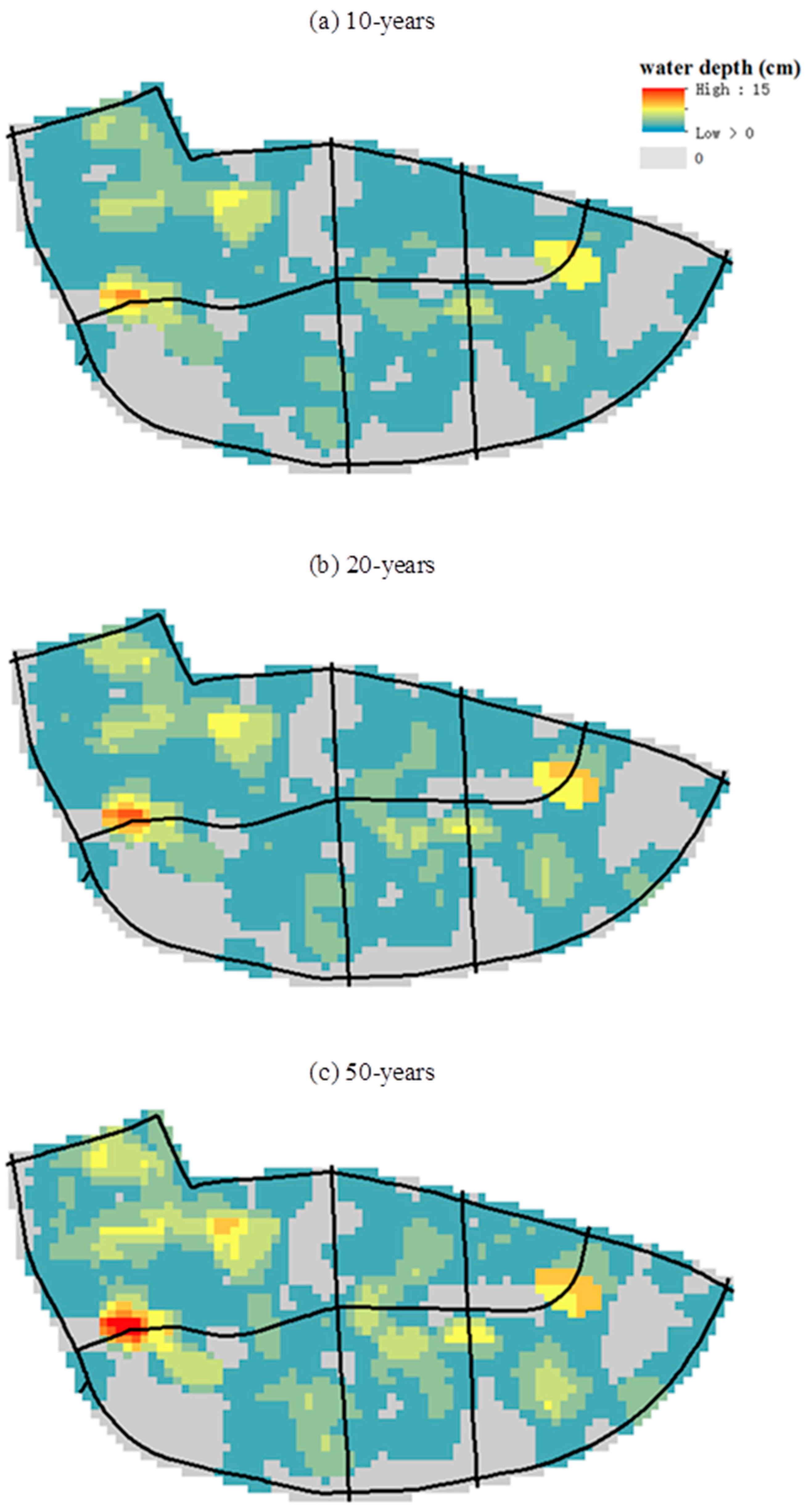
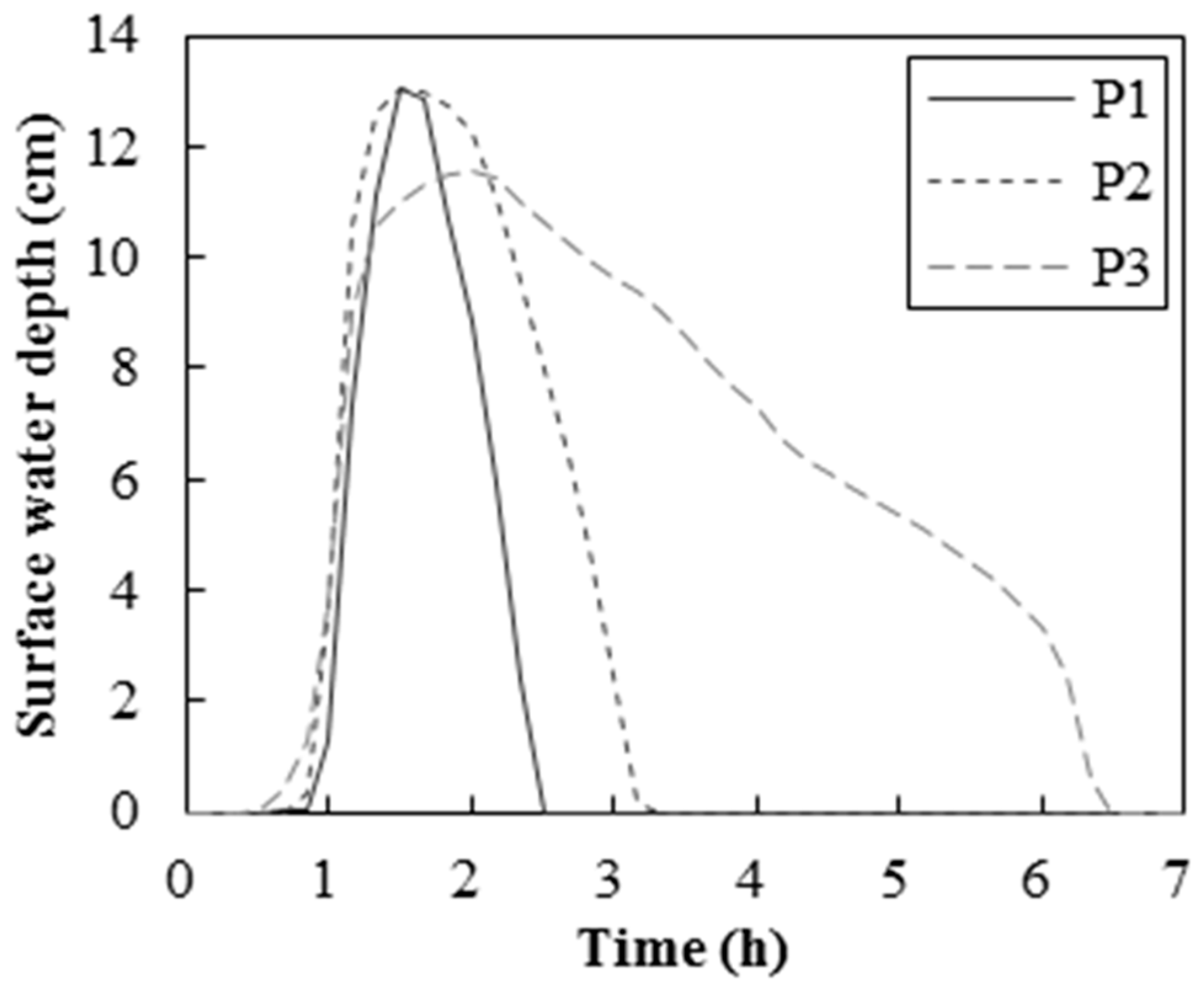
Figure 7 shows the water accumulation in the study area at the same time for different periods of regression. Clearly, with increasing rainfall intensity, the area of inundation is enlarged, and the depth of water accumulation increased. The variation of water depth in three selected areas is shown in Figure 8. It can be seen that all areas experienced a similar process of flood accumulation to a peak level, followed by recession. Nevertheless, the maximum depth and times of increase and decrease of the flood differed because of the characteristics of slope, permeability, and the drainage system.
4.2. Results of Traffic Simulation
We simulated the traffic situation dynamically using the 24-h traffic volume. As each vehicle in our study was deemed an agent, the number of agents is shown in Figure 9. The simulation results match the actual situation well.
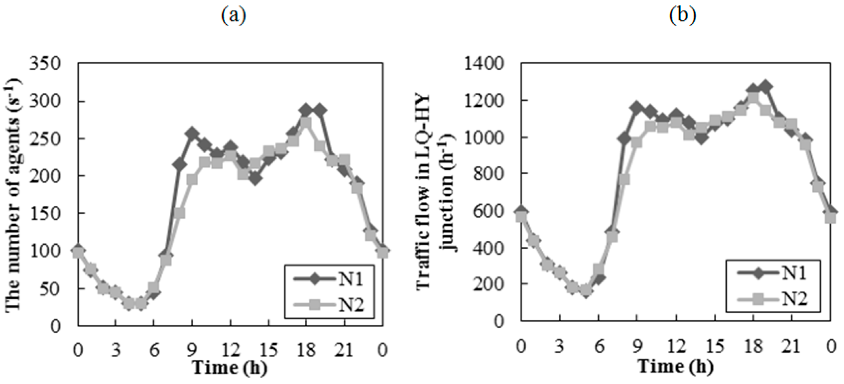
Based on traffic volume data from 26 June 2017 (Monday) and 25 June 2017 (Sunday), representative of the traffic conditions on a weekday and on the weekend, we simulated both situations and obtained the results shown in Figure 9. In this figure, the left panel represents the instantaneous number of agents per hour in the entire system, and the right panel represents the traffic volume passing through the intersection of Li Qing Road and Hua Yuan Road per hour. The trends of simulated traffic volume shown in both panels are similar to the actual data at all five intersections shown in Figure 4, indicating the reliability of this traffic simulation.
From Figure 9a, it is obvious that congestion on the weekday is more serious than on the weekend, especially in the morning. The level of congestion in both situations fluctuates within a certain range in the afternoon. For example, the traffic volumes at 14:00, 15:00, 16:00, 20:00, and 21:00 on the weekend were higher than during the same periods on weekdays. This finding is shown in Figure 9b, as the intersection of Li Qing Road and Hua Yuan Road is one of the main transport hubs in the entire system; it has an important role in concentrating and diffusing traffic. Consequently, the traffic volume at this junction from 09:00 to 22:00 remained high with little variation.
4.3. Crowding Degree under Different Storm Start Times
Here, the rainfall intensity is fixed, and the influence of the time of rainfall occurrence on the crowding degree is analyzed. Compared with the average crowding degree of the entire traffic system of the study area, P1 (labeled in Figure 2) presents a more serious condition. Because of the serious water accumulation in P1 over a long time and the high depth of water accumulation, the crowding degree study is significant.
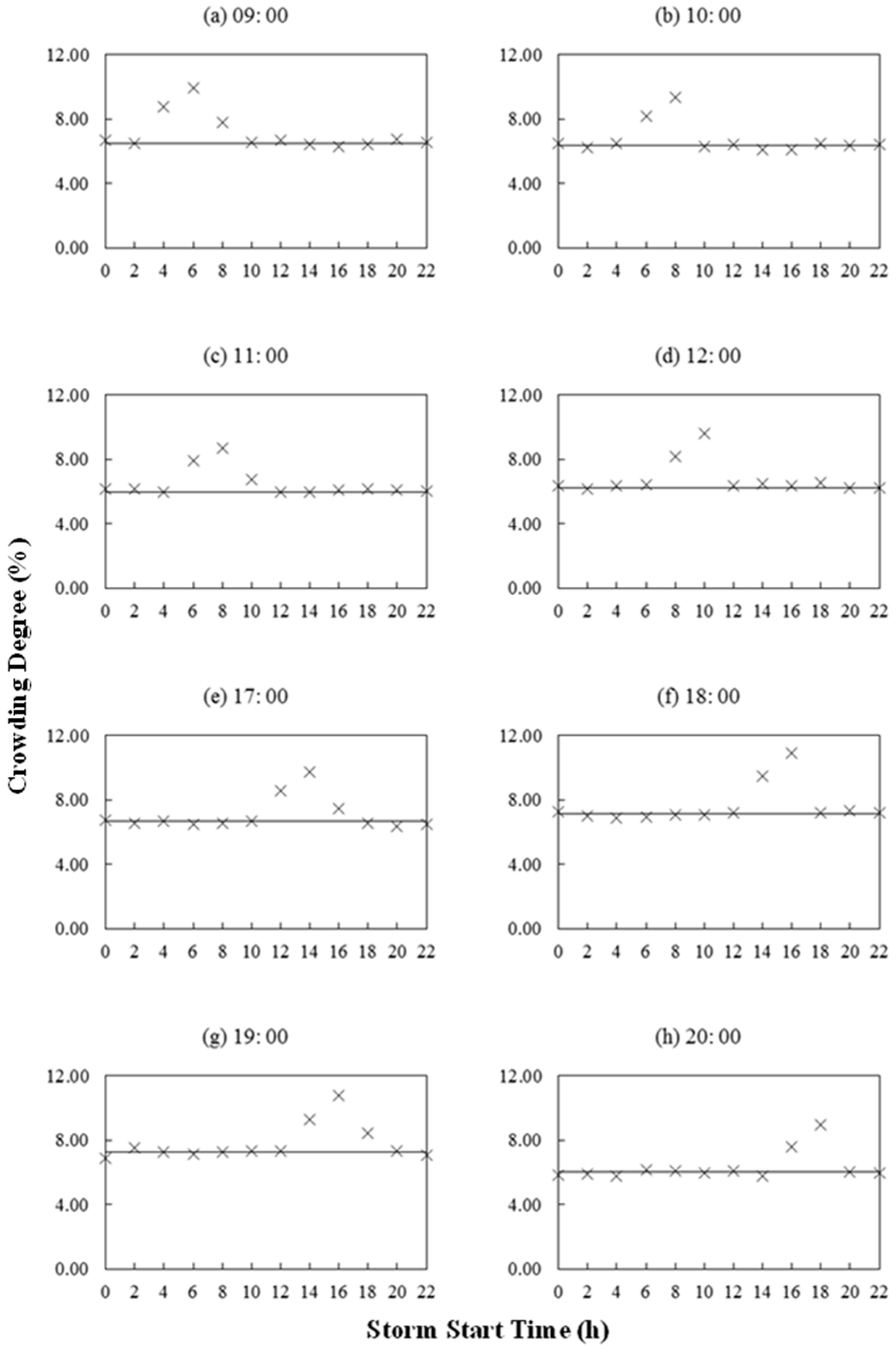
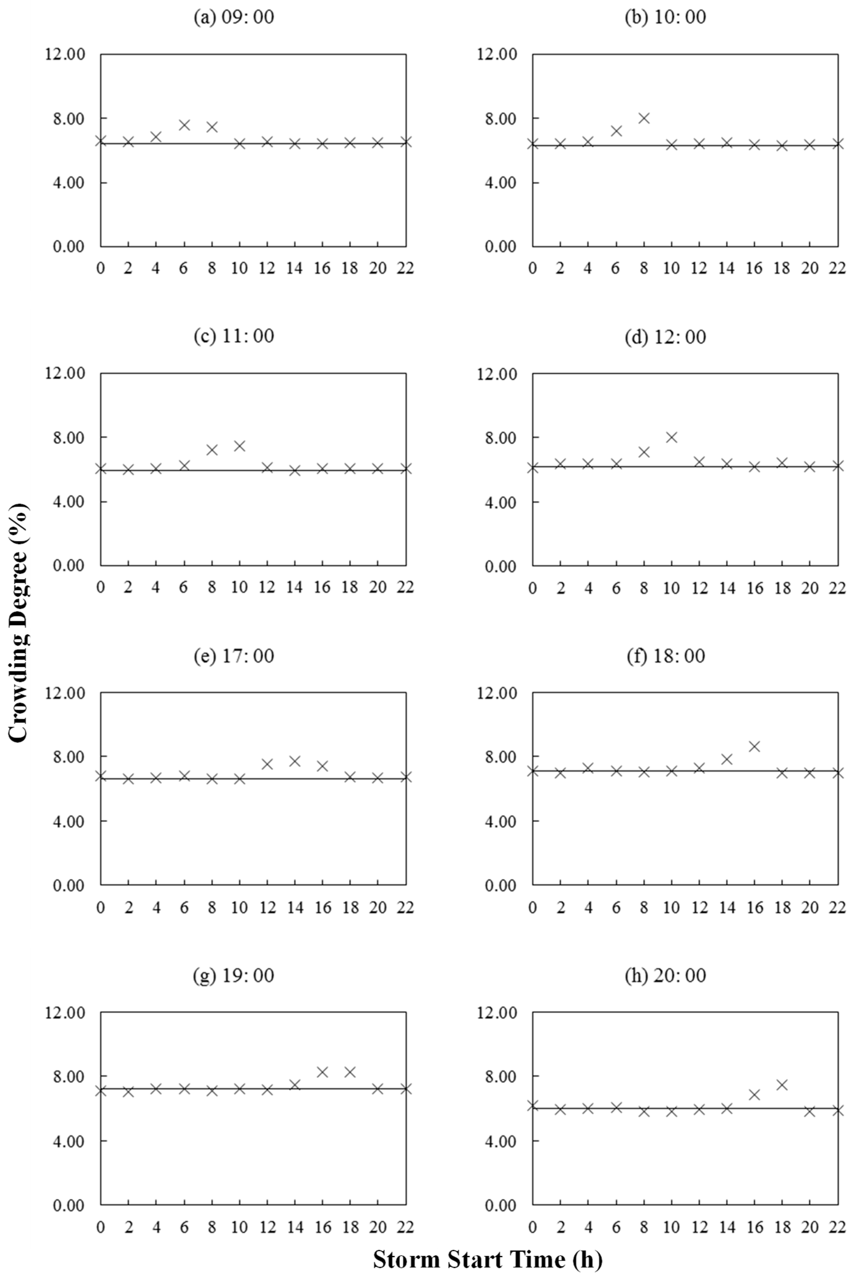
Figure 10 illustrates the case of RC (50 years) at P1 on Monday as an example. The abscissa represents the storm start time, and the ordinate shows the crowding degree. For ease of comparison, the crowding degree of a situation without flooding is represented as a straight line in the diagram. We selected 09:00, 10:00, 11:00, and 12:00 as four morning moments and 17:00, 18:00, 19:00, and 20:00 as evening moments.
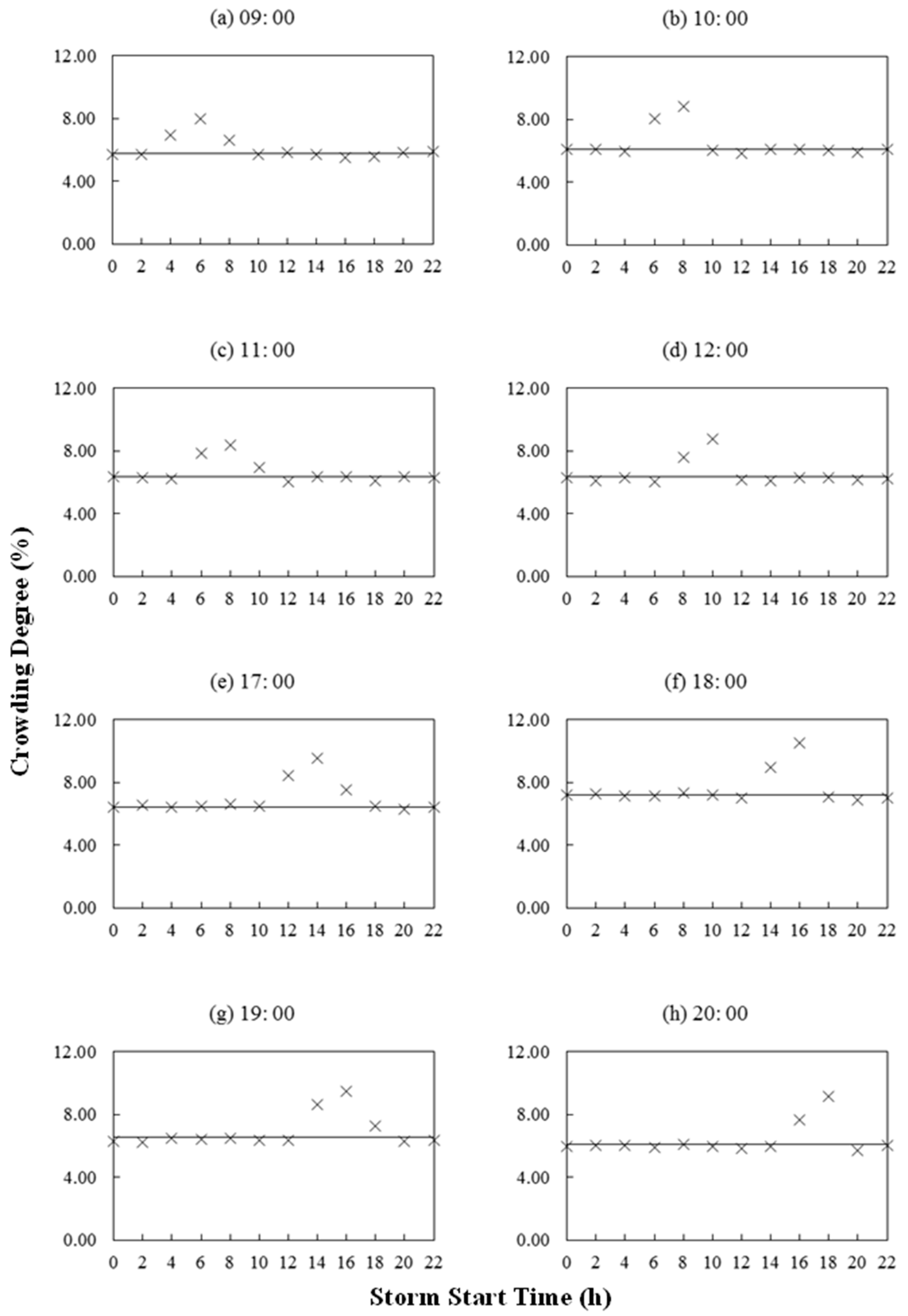
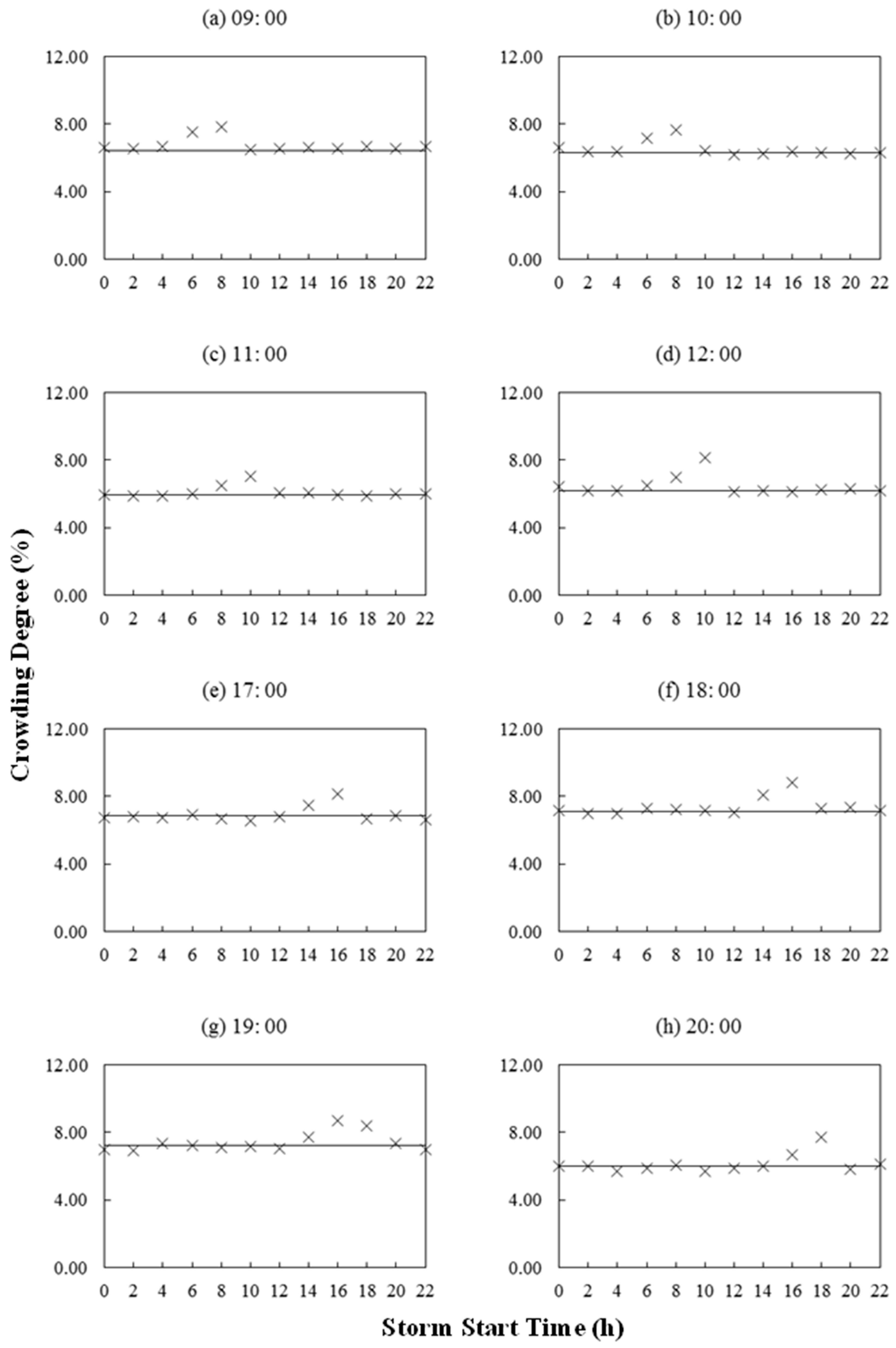
Figure 10a–d represent the crowding degree of P1 for different times of occurrence of rainfall during morning moments, while Figure 10e–h represent the crowding degree of P1 in evening moments. Figure 10a represents the impact of twelve different times of occurrence of rainfall on the crowding degree at 10:00 on Monday. It is evident that the traffic at 09:00 is only influenced notably when the rain starts at 04:00, 06:00, and 08:00. In particular, the rain that starts at 06:00 has the greatest influence, which approaches 10%, followed by the rain that starts at 04:00 and 08:00. The rainfall that occurs at other times shows a similar crowding degree with only a small fluctuation in amplitude. Figure 10b shows that the times of rainfall occurrence of 06:00 and 08:00 affect congestion seriously at P1. As can be seen when considering all the panels of Figure 10, the rain that occurs during the first five hours has a definite impact on road congestion and the greatest impact during the hour following the cessation of the rain. Similar conclusions can be reached for the weekend based on the trends shown in Figure 11.
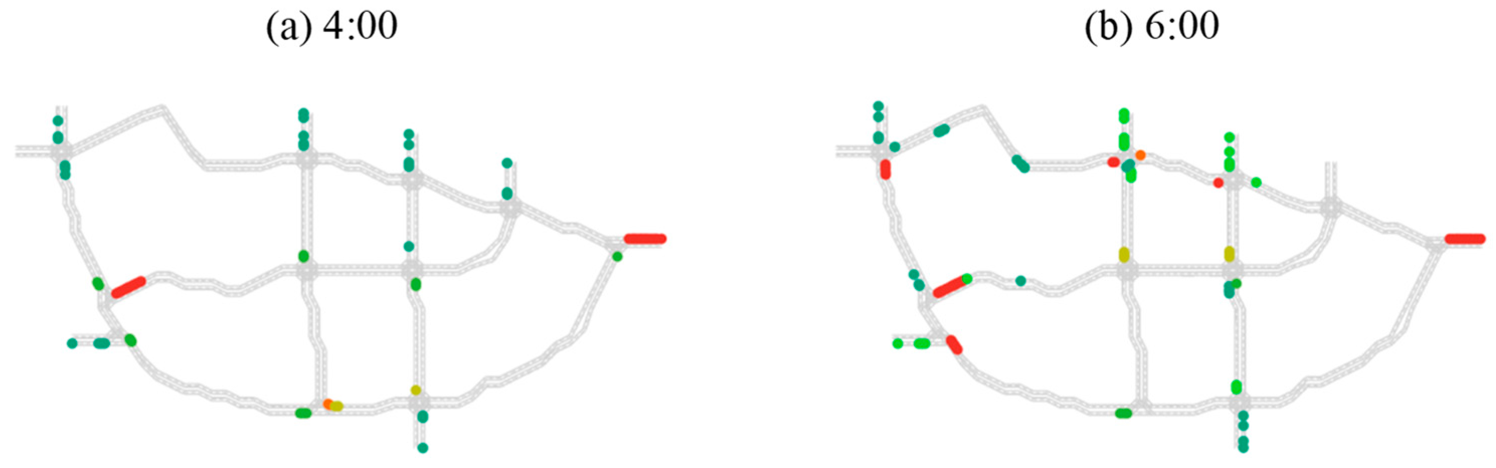
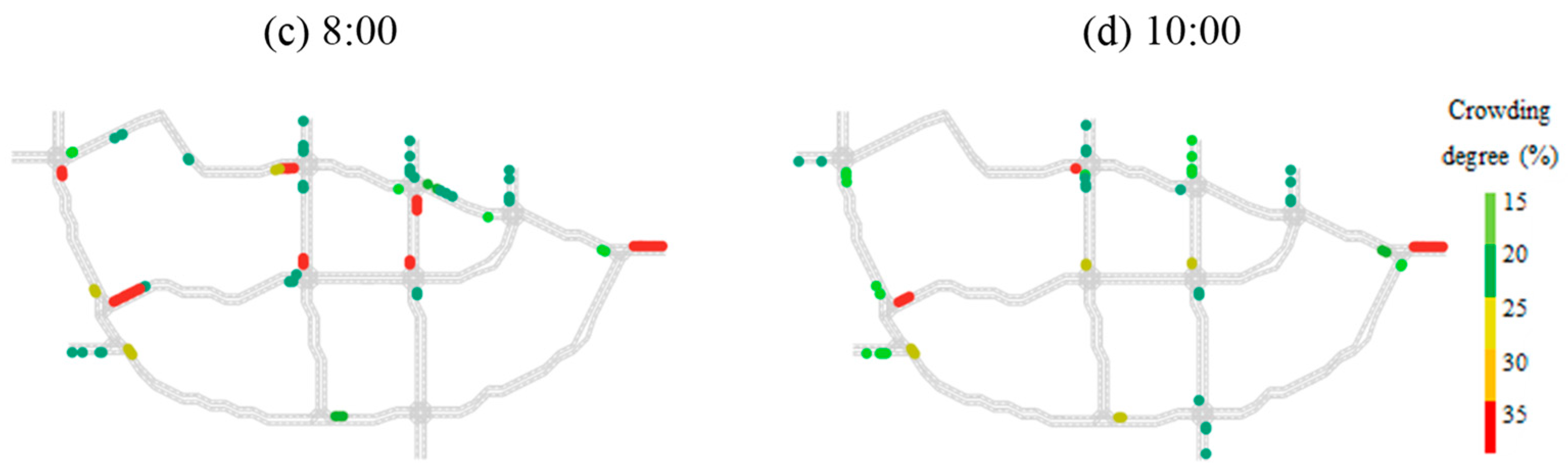
Comparison of the weekday and weekend situations, shown in Figure 10 and Figure 11, reveals that the morning weekday is crowded and that the influence of rainfall is serious. However, in the evening moments, the congestion of the two days appears similar. Overall, the traffic conditions on weekdays and on the weekend show considerable similarities. However, Figure 12a–d show the differences in the distribution of congestion at 10:00 for the four morning storm start times.
4.4. Crowding Degree under Different Rainfall Intensity
Different rainfall intensities were simulated by changing the rainfall return period. By analyzing the crowding degree under different rainfall intensities with the same time of rainfall occurrence, the relationship between the rainfall return period and the congestion situation was explored (Figure 13 and Figure 14).
Figure 10, Figure 13 and Figure 14 show that different rainfall intensities can cause different crowding degrees. However, at the same time, rainfall of greater intensity leads to a higher depth of accumulated water and a greater influence on the crowding degree. The impact of RC is significantly higher than that of either RA or RB, while the influence of RA and RB is similar. In addition, RC clearly has an effect on traffic congestion within one hour after the start of the rainfall, whereas RA and RB have little or no effect.
In Figure 10, Figure 13 and Figure 14, it can be found that different rainfall intensities result in different crowding degrees. However, there are strong and positive correlations among rainfall intensity, water depth, and the crowding degree. With an increase in rainfall intensity, water accumulates easily and the road becomes congested. The impact of RC is significantly higher than that of either RA or RB, while the influences of RA and RB are similar. In addition, RC has an obvious effect on the traffic congestion within an hour after the onset of rainfall, whereas RA and RB have hardly any effect.
5. Conclusions
Urban flooding has a considerable impact on driver behavior that makes traffic congestion more serious. This study proposed a method to analyze how urban floods might affect traffic congestion specifically. First, the spatial and temporal distributions of flooding were simulated by the SWMM–TELEMAC2D integrated model. Second, an ABM was established to simulate driver behavior patterns in the event of flooding using a car-following model. Finally, we combined the traffic and hydrologic simulation results and performed a detailed simulation of traffic conditions under flooding scenarios based on a case study of the Liandu District in Lishui.
The proposed method can predict flooding and traffic conditions in different places at different times, and it can also provide effective reference information in relation to public travel and urban disaster management. In summary, there were four main elements to this study. First, the TELEMAC-2D overland flow model was linked with the 1D SWMM sewer network model to undertake hydrologic simulations by the interaction of discharge and the synchronization of timing. The integrated model was found to be capable of achieving comprehensive consideration of the underground and surface water flows, and of obtaining predictions with different temporal and spatial distributions. Second, the space–time distribution of traffic was simulated using the ABM. Third, it was established that two-hour rainfall has a definite impact on traffic congestion over a five-hour period, with the greatest impact during an hour following the cessation of the rain. Finally, the effects of rainfall with 10- and 20-year return periods on the simulation were found to be similar and small, while the effect of rainfall with a 50-year return period was obvious.
It is worth noting that there is no complete way to validate the proposed method. This is because the parameters of human behavior and psychological processes are hard (or, to some extent, impossible) to obtain. We have tried to validate the proposed method through indirect methods. For example, the real traffic information at each road intersection was collected and compared with the simulated one. However, some problems remain unresolved. For example, great uncertainty remains regarding the use of the ABM itself, e.g., the different speeds of different vehicles under the same water depth, different starting points and destinations of the drivers, and different choices of direction by drivers at intersections. Consequently, each time the parameters involved in the simulation changed, the results obtained were different. In this study, our conclusions emphasize the average standard without any specific analysis regarding the influence of other parameters. In addition, the investigation of different storm durations on the proposed scheme is also an interesting topic. However, we cannot include all these studies in one paper. Therefore, in future studies, further work will be needed to optimize the proposed method, and the effect of different storm durations should also be considered.
Author Contributions
J.Z. was responsible for setting up the experiments, completing most of the experiments, and writing the initial draft of the manuscript. J.Z. and Y.D. modified the manuscript and contributed to the literature search. Q.D. and S.Z. principally conceived the idea for and design of the study and provided financial support. Y.D., A.Z., and Y.Z. processed the data.
Acknowledgments
This work was supported by the National Natural Science Foundation of China (Grant Nos. 41501429, 41771431), the Top-notch Academic Programs Project of Jiangsu Higher Education Institutions (TAPP), and the University Natural Science Project of Jiangsu Province (Grant No. 16KJA170001).
Conflicts of Interest
The authors declare no conflict of interest.
References
- Tang, T.Q.; Caccetta, L.; Wu, Y.H.; Huang, H.J.; Yang, X.B. A macro model for traffic flow on road networks with varying road conditions. J. Adv. Transp. 2014, 48, 304–317. [Google Scholar] [CrossRef]
- Greenshields, B.D. A study of traffic capacity. Highw. Res. Board Proc. 1935, 14, 448–477. [Google Scholar]
- Sugihakim, R.; Alatas, H. Application of a Boltzmann-entropy-like concept in an agent-based multilane traffic model. Phys. Lett. A 2016, 380, 147–155. [Google Scholar] [CrossRef]
- Manley, E.; Cheng, T.; Penn, A.; Emmonds, A. A framework for simulating large-scale complex urban traffic dynamics through hybrid agent-based modelling. Comput. Environ. Urban Syst. 2014, 44, 27–36. [Google Scholar] [CrossRef]
- Maroto, J.; Delso, E.; Felez, J.; Cabanellas, J.M. Real-Time Traffic Simulation with a Microscopic Model. IEEE Trans. Intell. Transp. Syst. 2006, 7, 513–527. [Google Scholar] [CrossRef]
- Newell, G.F. A simplified car-following theory: A lower order model. Transp. Res. Part B 2002, 36, 195–205. [Google Scholar] [CrossRef]
- Ward, J.A. Car-following models: Fifty years of linear stability analysis—A mathematical perspective. Transp. Plan. Technol. 2011, 34, 3–18. [Google Scholar]
- Yu, Y.; Kamel, A.E.; Gong, G.; Li, F. Multi-agent based modeling and simulation of microscopic traffic in virtual reality system. Simul. Model. Pract. Theory 2014, 45, 62–79. [Google Scholar] [CrossRef]
- Ben-Akiva, M.; Palma, A.D.; Kanaroglou, P. Dynamic Model of Peak Period Traffic Congestion with Elastic Arrival Rates. Transp. Sci. 1986, 20, 164–181. [Google Scholar] [CrossRef]
- Djordjević, S.; Prodanović, D.; Maksimović, C.; Ivetić, M.; Savić, D. SIPSON—Simulation of interaction between pipe flow and surface overland flow in networks. Water Sci. Technol. 2005, 52, 275–283. [Google Scholar] [PubMed]
- Leandro, J. Advanced Modelling of Flooding in Urban Areas: Integrated 1D/1D and 1D/2D Models; University of Exeter: Exeter, UK, 2008. [Google Scholar]
- DHI. MIKE-STORM. 2007. Available online: http://www.dhigroup.com/ (accessed on 16 September 2017).
- DHI. MIKE-21. 2007. Available online: http://www.dhigroup.com/ (accessed on 16 September 2017).
- Carr, R.S.; Smith, G.P. Linking of 2D and Pipe hydraulic models at fine spatial scales. Water Pract. Technol. 2007, 2. [Google Scholar] [CrossRef]
- Chen, S.H.; Djordjević, S.; Leandro, J.; Savić, D. The Urban Inundation Model with Bidirectional Flow Interaction between 2D Overland Surface and 1D Sewer Networks. 2007. Available online: http://hdl.handle.net/10871/16020 (accessed on 6 October 2017).
- Spry, R.; Zhang, S. Modelling of Drainage Systems and Overland Flowpaths at Catchment Scales. In Book of Proceedings: 7th International Conference on Urban Drainage Modelling and the 4th International Conference on Water Sensitive Urban Design; Monash University: Melbourne, Australia, 2006. [Google Scholar]
- Ata, R. Telemac2d User Manual, version 7.2. 2017. Available online: http://wiki.opentelemac.org/ (accessed on 29 September 2017).
- Cools, M.; Moons, E.; Wets, G. Assessing the Impact of Weather on Traffic Intensity. Weather Clim. Soc. 2008, 2, 60–68. [Google Scholar] [CrossRef]
- Lin, Q.; Nixon, W.A. Effects of Adverse Weather on Traffic Crashes: Systematic Review and Meta-Analysis. Transp. Res. Record J. Transp. Res. Board 2008, 2055, 139–146. [Google Scholar]
- Goodwin, L.C. Weather Impacts on Arterial Traffic Flow; Road Weather Management Program: Washington, DC, USA, 2002.
- Billot, R.; Faouzi, N.E.E.; Vuyst, F.D. Multilevel Assessment of the Impact of Rain on Drivers’ Behavior. Transp. Res. Record J. Transp. Res. Board 2009, 2107, 134–142. [Google Scholar] [CrossRef]
- Su, B.; Huang, H.; Li, Y. Integrated simulation method for waterlogging and traffic congestion under urban rainstorms. Nat. Hazards 2016, 81, 23–40. [Google Scholar] [CrossRef]
- Leandro, J.; Martins, R. A methodology for linking 2D overland flow models with the sewer network model SWMM 5.1 based on dynamic link libraries. Water Sci. Technol. 2016, 73, 3017–3026. [Google Scholar] [CrossRef] [PubMed]
- Chen, A.S.; Leandro, J.; Djordjeviä, S. Modelling sewer discharge via displacement of manhole covers during flood events using 1D/2D SIPSON/P-DWave dual drainage simulations. Urban Water J. 2015, 13, 830–840. [Google Scholar] [CrossRef]
- Rossman, L.E. SWMM 5.0 Manual; EPA/600/R-05/040; CHI Press: Cincinnati, OH, USA, 2008. [Google Scholar]
- Fernandes, E.H.; Dyer, K.R.; Niencheski, L.F.H. Calibration and Validation of the TELEMAC-2D Model to the Patos Lagoon (Brazil). J. Coast. Res. 2001, 34, 470–488. [Google Scholar]
- House-Peters, L.A.; Chang, H. Urban water demand modeling: Review of concepts, methods, and organizing principles. Water Resour. Res. 2011, 47, 1837–1840. [Google Scholar] [CrossRef]
- Wilensky, U.; Stroup, W. Netlogo User Manual; Center for Connected Learning and Computer-Based Modeling, Northwestern University: Evanston, IL, USA, 1999. [Google Scholar]
- Nasello, C.; Tucciarelli, T. Dual Multilevel Urban Drainage Model. J. Hydraul. Eng. 2005, 131, 748–754. [Google Scholar] [CrossRef]
- Reuschel, A. Vehicle movements in a platoon. Oesterreichisches Ingenieur-Archir 1950, 4, 193–215. [Google Scholar]
- Chandler, R.E.; Herman, R.; Montroll, E.W. Traffic Dynamics: Studies in Car Following. Oper. Res. 1958, 6, 165–184. [Google Scholar] [CrossRef]
- Kometani, E.; Sasaki, T. Dynamic Behaviour of Traffic with a Nonlinear Spacing-Speed Relationship; Elsevier Publishing Co.: Amsterdam, The Netherlands, 1959. [Google Scholar]
- Krauß, S. Microscopic Modeling of Traffic Flow: Investigation of Collision Free Vehicle Dynamics; University of Cologne: Cologne, Germany, 1998. [Google Scholar]
- Chowdhury, D.; Santen, L.; Schadschneider, A. Statistical physics of vehicular traffic and some related systems. Phys. Rep. 2000, 329, 199–329. [Google Scholar] [CrossRef]
- Oluwaseyi, O.S.; Adebola, O.; Edwin, K.A.; Okoko, E.E.; Stephen, M. Examination of On-Street Parking and Traffic Congestion Problems in Lokoja. J. Rheumatol. 2014, 27, 1336–1342. [Google Scholar]
- Cen, G.; Shen, J.; Fan, R. Research on Rainfall Pattern of Urban Design Storm. Adv. Water Sci. 1998, 9, 41–46. [Google Scholar]
Figure 1.
Map showing the general location of the study area (left) and the digital elevation model map displaying specific details of the study area (right).
Figure 1.
Map showing the general location of the study area (left) and the digital elevation model map displaying specific details of the study area (right).

Figure 2.
Remote sensing image of the study area showing the main road network and locations of five traffic flow monitors (P1, P2, and P3 indicate three locations of serious flooding).
Figure 2.
Remote sensing image of the study area showing the main road network and locations of five traffic flow monitors (P1, P2, and P3 indicate three locations of serious flooding).

Figure 3.
Structure of the drainage system in the study area.

Figure 4.
Traffic flow on Monday, 3 July 2017, without rain.

Figure 5.
Modeled junction structure at a crossroads. The direction of each unidirectional road is represented by an arrow. The colored nodes change color to reflect the condition of the traffic lights.
Figure 5.
Modeled junction structure at a crossroads. The direction of each unidirectional road is represented by an arrow. The colored nodes change color to reflect the condition of the traffic lights.

Figure 6.
Method of direction selection at a junction (using a crossroads as an example).

Figure 7.
Map of accumulated water depth (1 h 30 min after the rain occurrence) (a) 50-year return period; (b) 50-year return period; (c) 50-year return period.
Figure 7.
Map of accumulated water depth (1 h 30 min after the rain occurrence) (a) 50-year return period; (b) 50-year return period; (c) 50-year return period.

Figure 8.
Change of the surface water depth in three areas (labeled in Figure 1) of serious flooding (origin indicates time of rain onset).
Figure 8.
Change of the surface water depth in three areas (labeled in Figure 1) of serious flooding (origin indicates time of rain onset).

Figure 9.
Results of traffic simulation. (a) Number of agents at each hour in the entire system and (b) traffic flow at LQ–HY junction per hour.
Figure 9.
Results of traffic simulation. (a) Number of agents at each hour in the entire system and (b) traffic flow at LQ–HY junction per hour.

Figure 10.
Results of crowding degree for different storm start times of RC (50 years) on a weekday (Monday) at P1. Each panel represents a moment: (a–d) show morning moments and (e–h) show evening moments.
Figure 10.
Results of crowding degree for different storm start times of RC (50 years) on a weekday (Monday) at P1. Each panel represents a moment: (a–d) show morning moments and (e–h) show evening moments.

Figure 11.
Results of crowding degree for different storm start times of RC (50 years) on the weekend (Sunday) at P1. Each panel represents a moment: (a–d) show morning moments and (e–h) show evening moments.
Figure 11.
Results of crowding degree for different storm start times of RC (50 years) on the weekend (Sunday) at P1. Each panel represents a moment: (a–d) show morning moments and (e–h) show evening moments.

Figure 12.
Distribution of congestion for the four storms’ start times at 10:00. Each panel represents a storm start time: (a) 4: 00; (b) 6:00; (c) 8: 00; (d) 10:00.
Figure 12.
Distribution of congestion for the four storms’ start times at 10:00. Each panel represents a storm start time: (a) 4: 00; (b) 6:00; (c) 8: 00; (d) 10:00.


Figure 13.
Results of crowding degree for different storm start times of RA (10 years) on the weekday (Monday) at P1. Each panel represents a moment: (a–d) show morning moments and (e–h) show evening moments.
Figure 13.
Results of crowding degree for different storm start times of RA (10 years) on the weekday (Monday) at P1. Each panel represents a moment: (a–d) show morning moments and (e–h) show evening moments.

Figure 14.
Results of crowding degree for different storm start times of RB (20 years) on the weekday (Monday) at P1. Each panel represents a moment: (a–d) show morning moments and (e–h) show evening moments.
Figure 14.
Results of crowding degree for different storm start times of RB (20 years) on the weekday (Monday) at P1. Each panel represents a moment: (a–d) show morning moments and (e–h) show evening moments.


Table 1.
Average speed (km/h) based on several attributes.
| Attribute | Water Depth (cm) | |||
|---|---|---|---|---|
| 0 | 10 | 20 | 30 | |
| Male, Age < 35 | 50.9 | 38.4 | 27.6 | 16.9 |
| Male, Age ≥ 35 | 49.8 | 37.1 | 26.0 | 14.9 |
| Female, Age < 35 | 50.8 | 37.5 | 26.0 | 14.4 |
| Female, Age ≥ 35 | 49.8 | 36.1 | 24.3 | 12.5 |
Table 2.
Parameter variations used in the simulation scenarios. (“Rainfall Return Period” in Group N corresponds to simulation time).
Table 2.
Parameter variations used in the simulation scenarios. (“Rainfall Return Period” in Group N corresponds to simulation time).
| Scenarios | Rainfall Return Periods | Weekdays or Weekends |
|---|---|---|
| RA1 | 10 years | Weekdays |
| RA2 | 10 years | Weekends |
| RB1 | 20 years | Weekdays |
| RB2 | 20 years | Weekends |
| RC1 | 50 years | Weekdays |
| RC2 | 50 years | Weekends |
| N1 | No rain | Weekdays |
| N2 | No rain | Weekends |
Note: R and N represent rain and no rain, respectively; A, B, and C indicate different rainfall return periods, and numbers (1, 2) are used to distinguish weekdays and weekends.
© 2018 by the authors. Licensee MDPI, Basel, Switzerland. This article is an open access article distributed under the terms and conditions of the Creative Commons Attribution (CC BY) license (http://creativecommons.org/licenses/by/4.0/).
Share and Cite
MDPI and ACS Style
Zhu, J.; Dai, Q.; Deng, Y.; Zhang, A.; Zhang, Y.; Zhang, S. Indirect Damage of Urban Flooding: Investigation of Flood-Induced Traffic Congestion Using Dynamic Modeling. Water 2018, 10, 622. https://doi.org/10.3390/w10050622
AMA Style
Zhu J, Dai Q, Deng Y, Zhang A, Zhang Y, Zhang S. Indirect Damage of Urban Flooding: Investigation of Flood-Induced Traffic Congestion Using Dynamic Modeling. Water. 2018; 10(5):622. https://doi.org/10.3390/w10050622
Chicago/Turabian StyleZhu, Jingxuan, Qiang Dai, Yinghui Deng, Aorui Zhang, Yingzhe Zhang, and Shuliang Zhang. 2018. "Indirect Damage of Urban Flooding: Investigation of Flood-Induced Traffic Congestion Using Dynamic Modeling" Water 10, no. 5: 622. https://doi.org/10.3390/w10050622
Note that from the first issue of 2016, this journal uses article numbers instead of page numbers. See further details here.