Article

A Simulation-Based Linear Fractional Programming Model for Adaptable Water Allocation Planning in the Main Stream of the Songhua River Basin, China

1
School of Water Conservancy & Civil Engineering, Northeast Agricultural University, Harbin 150030, China
2
Key Laboratory of Effective Utilization of Agricultural Water Resources of Ministry of Agriculture, Northeast Agricultural University, Harbin 150030, China
3
Heilongjiang Provincial Key Laboratory of Water Resources and Water Conservancy Engineering in Cold Region, Northeast Agricultural University, Harbin 150030, China
*
Author to whom correspondence should be addressed.
Water 2018, 10(5), 627; https://doi.org/10.3390/w10050627
Submission received: 26 April 2018 / Revised: 5 May 2018 / Accepted: 7 May 2018 / Published: 10 May 2018
(This article belongs to the Section Water Resources Management, Policy and Governance)

Abstract

:
The potential influence of natural variations in a climate system on global warming can change the hydrological cycle and threaten current strategies of water management. A simulation-based linear fractional programming (SLFP) model, which integrates a runoff simulation model (RSM) into a linear fractional programming (LFP) framework, is developed for optimal water resource planning. The SLFP model has multiple objectives such as benefit maximization and water supply minimization, balancing water conflicts among various water demand sectors, and addressing complexities of water resource allocation system. Lingo and Excel programming solutions were used to solve the model. Water resources in the main stream basin of the Songhua River are allocated for 4 water demand sectors in 8 regions during two planning periods under different scenarios. Results show that the increase or decrease of water supply to the domestic sector is related to the change in population density at different regions in different target years. In 2030, the water allocation in the industrial sector decreased by 1.03–3.52% compared with that in 2020, while the water allocation in the environmental sector increased by 0.12–1.29%. Agricultural water supply accounts for 54.79–77.68% of total water supply in different regions. These changes in water resource allocation for various sectors were affected by different scenarios in 2020; however, water resource allocation for each sector was relatively stable under different scenarios in 2030. These results suggest that the developed SLFP model can help to improve the adjustment of water use structure and water utilization efficiency.

1. Introduction

Most surface water resources are stored in channels and basins, and these waters have long regeneration cycles and are heterogeneously distributed. The impact of global warming on future water resources cannot be neglected in the process of developing and utilizing these resources [1]. Specifically, researchers and managers have to determine how to allocate limited water resources to different areas or water departments to achieve the optimal balance between social, economic and ecological benefits. Thus, optimizing water resource allocation is an important task [2,3,4].
With the development of economy and society, the development and utilization of water resources has gradually shifted from a single goal to a comprehensive utilization. Under such circumstances, the single objective programming method that focuses on economic benefit only is no longer applicable. Optimal water resource allocation involves many aspects such as the social economy, ecological environment, etc. In order to improve the efficiency of water resource allocation and avoid the contradiction of water resource utilization between different water demand sectors, it is necessary to adopt multi-objective programming to planning water resources. Multi-objective programming considers two or more targets and makes alternatives for conflicting finite (infinite) schemes simultaneously. Many experts and scholars have adopted multi-objective programming methods to solve the problem of optimal water resource allocation [5,6,7,8,9]. As an effective method for handling multi-objective problems, linear fractional programming (LFP), which can also affect system efficiency quantificationally, has been used recently in water resource allocation. For example, Zhang et al. [10] developed a model that can be derived from integrating generalized fuzzy credibility-constrained programming (GFCCP) into a linear fractional programming (LFP) optimization framework to optimize water resources. Mani et al. [11] formulated a conjunctive-use model for the management of groundwater and surface water via mixed integer linear fractional programming. Ren et al. [12] combined an LFP model and a chance constrained programming (CCP) model to determine whether the water resource carrying capacity of Jinchang City could meet the requirements of economic development. However, the LFP, which falls within the capability of linear fractional programming in a multi-objective framework, and the runoff simulation model (RSM) have been applied to optimal water allocation in limited cases.
Water resource planning is important to provide a reference for water resource management in the future. Water resource planning is strongly affected by runoff. Therefore, runoff forecasting is necessary when planning water resources. Runoff forecasting is constrained by climate change. The Intergovernmental Panel on Climate Change (IPCC) is the international body for assessing the science related to climate change. Since its inception in 1988, the IPCC has completed five assessment reports [13,14,15]. These reports have provided the main scientific basis for the international community to understand and investigate climate change. Many global scholars have used different climate models in the Coupled Model Intercomparison Project Phase 5 (CMIP5) to simulate and evaluate the future climate in various regions of the world [16,17,18,19]. There is a strong consensus regarding the changes in climate caused by increased concentrations of anthropogenic greenhouse gas emissions, and the subsequent effects of climate change on runoff are inevitable [20]. Precipitation and temperature are the main elements that influence climate change and runoff variation. The vertical and lateral redistribution of water in the subsurface is influenced by annual and interannual variations in precipitation, and the calculation of potential evaporation (PET) directly reflects the effect of temperature on runoff [21]. Recently, numerous studies on runoff forecasting considering climate change have been conducted [22,23,24,25]. Unfortunately, information on how the changes in precipitation and temperature affect runoff forecasting and thus affect water allocation efficiency considering the economic benefit maximization and water supply minimization simultaneously is limited.
Therefore, the aim of this study is the development of a simulation-based linear fractional programming model for adaptable water allocation planning. The SLFP model developed in this paper combines the runoff simulation model (RSM) and LFP model to provide a reasonable scheme for the optimal allocation of water resources in the future. The objective of the SLFP model is to allocate available water resources to different water sectors in various regions to improve the utilization efficiency of water resources and provide evidence for water resource planning under climate change. The developed model is then applied in a real-world case study in the main stream basin of the Songhua River, Northeast China. The optimal allocation of water resources is estimated in different periods based on various temperature and precipitation scenarios, which can be used for providing information on the balance among different departments, allocation strategies, and agriculture sustainability.

2. Data and Methodology

2.1. Study Area and Data

The Songhua River basin is located in Northeast China. The Songhua River is one of the seven major rivers in China and the largest tributary of the Heilongjiang River. The river spans Inner Mongolia, Jilin and Heilongjiang Provinces. The study area includes the main stream of the Songhua River basin, which begins in Zhaoyuan County. Zhaoyuan County is the intersection of the Nenjiang River, Songhua River and second Songhua River. The main channel ends in Tongjiang City at the intersection of the Songhua River and Heilongjiang River (Figure 1). The Songhua River basin has a temperate monsoon climate and four distinct seasons. In the flood season (June-September), the precipitation is 397.5 mm, which is 60–80% of the annual precipitation, the mean air temperature is 19.4 °C, and the mean runoff is 29.19 billion m3 in the study area. Average daily precipitation, air temperature and flow data during the flood season from 1961 to 2010 are available for the study area: average daily precipitation and air temperature data were collected from 5 meteorological stations from 1961–2015 from the China Meteorological Data Service Center (http://data.cma.cn/). Additionally, average daily solar radiation data were derived from the National Earth System Science Data Sharing Infrastructure, National Science & Technology Infrastructure of China (http://www.geodata.cn). The corresponding data are shown in Table 1.

2.2. Methodology

2.2.1. Runoff Simulation Model

In order to better plan the water resources of the basin, runoff simulation is critical. In terms of this study, runoff has a direct relationship with precipitation and PET. This paper uses the relationship between runoff, precipitation and PET proposed by Liu [26], and it can be expressed as follows [27]:
R 0 = k P α P E T β
where R0 is the simulated runoff, 108 m3; P is the precipitation, mm; PET is the potential evapotranspiration, mm.

Precipitation

The average daily precipitation data in the flood season were collected from 5 meteorological stations from 1961–2015 from the National Meteorological Science Data Sharing Infrastructure (http://data.cma.cn/). By adding daily precipitation in the flood season, the precipitation in flood season for the 5 meteorological stations is obtained.

Potential Evaporation (PET)

Many computational methods of calculating PET are applicable, corresponding to different conditions [28,29,30,31,32]. According to the geographical characteristics of the study area and the selection of model parameters, the Makkink method is used to calculate the PET in this paper because it can estimate evapotranspiration in humid grassland areas. Makkink [28] proposed the Makkink formula in Holland, and it is a revised version of the [33] formula. The Makkink formula can be expressed as follows:
P E T = 0.61 Δ Δ + γ R S λ 0.12
where PET is the potential evapotranspiration, mm day−1; RS is the solar radiation, MJ m−2 day−1; Δ is the slope of the saturation vapour pressure curve, kPa °C−1; γ is the psychrometric constant; and λ is the latent heat of vaporization.
The slope of the saturation vapour pressure curve can be calculated using the following equation [34]:
Δ = 4098 × e o ( T + 237.3 ) 2
e o = exp [ 16.78 × T 116.9 T + 237.3 ]
where e o is the saturation vapour pressure on a given day, kPa, and T is the mean daily air temperature, °C.
The psychrometric constant can be determined as follows:
γ = c p × P s 0.622 × λ
where c p is the specific heat of moist air at a constant pressure, 1.013 × 10⁻³ MJ kg−1 °C−1, and Ps is the atmospheric pressure, kPa.
The latent heat of vaporization can be determined from the following expression.
λ = 2.501 2.361 × 10 3 × T
Finally, atmospheric pressure can be expressed as follows:
P s = 101.3 0.01152 E L + 0.544 × 10 6 × E L
where EL is the elevation, m.
This paper employs empirical relationships taken from Neitsch [34], applicable in the region under study. The calculated slope of the saturation vapour pressure curve and other parameters are consistent with the results of such studies in the same area [35,36] and show that Equations (3)–(7) are reasonable.

Model Evaluation

The reliability of the model is evaluated based on the relative error (RE) and the correlation coefficient (CC). The RE reflects the credibility of the RSM, and the CC reflects the overall efficiency of the RSM:
R E i = | R i G i | G i × 100 %
C C = i = 1 n ( G i G ¯ ) ( R i R ¯ ) i = 1 n ( G i G ¯ ) 2 i = 1 n ( R i R ¯ ) 2
where Gi is the measured value of the flood season runoff, G ¯ is the mean measured value of the flood season runoff; Ri is the simulated value of the flood season runoff, and R ¯ is the mean simulated value of the flood season runoff. The range of CC is 0–1, and the larger the CC, the better the model simulation capability and higher the efficiency, n is the total years, i represents the year.

2.2.2. Linear Fractional Programming

Linear-fractional programming (LFP) is a generalization of linear programming (LP). LFP represents optimization problems using linear equations and linear inequalities and has a richer set of objective functions. LFP can effectively reflect the efficiency of a system. Therefore, this method has certain advantages in optimizing water resources [37]. The common LFP model (denoted as primal programming, or PP) [38] can be expressed as follows:
{ max f ( x ) = c x + α d x + β A x b x 0
where A is an m by n matrix; x and b are column vectors with n and m components, respectively; c and d are row vectors with n components; α and β are constants; and d x + β > 0 .
A PP can be solved using dual theory, and the dual model is expressed as follows (denoted as dual programming, or DP).
{ min g ( y , z ) = z A T y + d T z c T b T y + β z = α y 0
Equation (10) is a linear model, and its optimal solution is ( y ^ , z ^ ) , which can be easily obtained by introducing the relaxation column vector, v ^ . In this case, v ^ = a T y ^ + d T z ^ - c T , and v ^ 0 . If x ^ is the optimal solution of Equation (10) and u ^ is a relaxation column vector, then a x ^ + u ^ = b and u ^ 0 . According to the relaxation theorem, if x ^ j v ^ j = 0 and y ^ j u ^ j = 0 , Equations (10) and (11) have the same optimal solution. Therefore, the LFP model can be solved with the above transformation.

2.2.3. Simulation-Based Linear Fractional Programming for Adaptable Water Allocation Planning

According to the conditions in the study area, The RSM is incorporated into the LFP model to form an optimal allocation model of water resources considering runoff variations, in which the runoff that is simulated by the RSM can be used as a constraint in the LFP model. The SLFP model considers changes in temperature and precipitation to effectively simulate real-world scenarios. The framework of the developed SLFP model is depicted in Figure 2.
The SLFP model aims to allocate limited water resources to different water demand sectors including the agricultural water sector, industrial water sector, domestic water sector and environmental water sector, which are denoted as AgWSit, InWSit, DoWSit, and EcWSit, respectively, in 2020 and 2030, denoted as t = 1 and t = 2, respectively. These four decision variables are limited by Chemical Oxygen Demand (COD), water resources and happiness index constraints. Equation (17) is a fractional programming model which reflects the maximization of system efficiency. Equation (12) is the numerator of Equation (17), which represents the maximization of the system’s economic benefits. Equation (16) is the denominator of Equation (17) that represents the minimum water supply of the system. The SLFP model can be written as follows.
Objective function:
max f 1 = A B C
A = t = 1 2 i = 1 8 ( I n V i t × I n W S i t + A g V i t × A g W S i t + E c V i t × E c W S i t )
B = t = 1 2 i = 1 8 ( D S O C t × D S T R t × D S D t × W S P i t × D o W S i t + I W O C t × I W T R t × I W D t × I n V i t × I n W S i t )
C = t = 1 2 R S T C O D t i = 1 8 ( O C D C O D t × D o C O D t × W S P i t × D o W S i t + O C I C O D t × I n C O D t × I n V i t × I n W S i t + O C A C O D t × A g C O D t × A g V i t × A g W S i t )
min f 2 = t = 1 2 i = 1 8 ( D o W S i t + I n W S i t + A g W S i t + E c W S i t )
max F = max f 1 min f 2
This model is subject to the following constraints:
Chemical Oxygen Demand (COD) constraints:
COD is the most used pollution index commonly. COD can reflect the degree of pollution in water. The greater the chemical oxygen demand, the more serious the pollution of organics in water. If COD is used as a constraint, the SLFP model can provide optimal water resource planning under the water quality standards.
( 1 R S T C O D t ) i = 1 8 ( W S P i t × D o W S i t × D o C O D t + I n V i t × I n W S i t × I n C O D t + A g V i t × A g W S i t × A g C O D t ) E c C O D t
Water resource constraints:
R0i is the connection point of RSM and LFP, and is obtained by RSM. It is also a constraint in the LFP model.
D o W S i t + I n W S i t + A g W S i t + E c W S i t R 0 i × 1 W U R t
{ min D o W S i t D o W S i t min I n W S i t I n W S i t min A g W S i t A g W S i t min E c W S i t E c W S i t
Happiness index constraints:
According to the outline of the thirteenth Five-Year plan of national economic and social development in Heilongjiang Province, primary and tertiary industries have developed rapidly, and the structure of the secondary industry has undergone various changes. The proportions of the three industrial sectors changed from 12.6:48.4:39 at the end of the 11th Five-Year to 17.5:31.8:50.7, and the ratio of industrial value added to agricultural value added dropped from 3.84 to 1.82. Observed and calculated ratio changes of the industrial value added and agricultural value added were obtained for the recent five-year plans. It is predicted that this ratio will fluctuate from 1.735 to 1.817 in 2020 and will fluctuate from 1.654 to 1.735 in 2030. The happiness index was established according to Engel’s Coefficient, the structural adjustment and future requirements for national happiness promotion. By calculating the ratio of per capita food consumption to total per capita consumption in the recent ten years, this ratio will fluctuate between 0.207 and 0.234 in 2020 and fluctuate between 0.186 and 0.207 in 2030. Therefore, the following restrictions are proposed to adjust the proportion of water allocation in different water demand sectors.
When t = 1:
0.207 A g V i t × A g W S i t C C E i t 0.234
When t = 2:
1.654 I n V i t × I n W S i t A g V i t × A g W S i t 1.735
0.186 A g V i t × A g W S i t C C E i t 0.207
A represents the value of total water output, yuan. A is made up of industry, agriculture and ecology added value, because domestic water does not produce added value. B represents the sewage treatment costs in sewage treatment plants, yuan. The equation assumes that agricultural wastewater treats only COD, and ecological water does not produce waste water. Therefore, B is made up of domestic and industrial sewage treatment costs. C represents the COD treatment costs, yuan. C is made up of domestic, industrial and agricultural COD treatment costs. The objective function represents the best ratio of economic benefit and water resource allocation. The above symbols are defined in Table 2.

3. Results and Analysis

3.1. Mann-Kendall Trend Test of Temperature, Precipitation and Runoff

The temperature in the study area increased from 1961 to 2015 based on the trend test results (Figure 3). The moving average curve of five years clearly showed the trend of temperature, precipitation and runoff. Specifically, the Mann-Kendall test showed that the statistic positive sequence curve (UF) and statistic inverse sequence curve (UB) of each region intersected in the 1990s, indicating that the temperature trend changed in the 1990s at a confidence level of 0.05, and the UF curve exceeded the critical value in 2005; therefore, the temperature in the study area exhibited a significant upward trend. Figure 3 shows the precipitation trends in the five regions from 1961 to 2015. Although there were relatively consistent fluctuations in overall change, there was no significant change in regularity. As shown in Figure 3, runoff in the five regions of the study area exhibited an increasing-decreasing-increasing-decreasing trend from 1961 to 2015. Additionally, the UF and UB curves of runoff in each region intersected in the 1990s, indicating that the runoff trend changes in the 1990s at a confidence level of 0.05. This result suggests that the decrease in runoff and increase in air temperature were not only related but also synchronous.

3.2. Runoff Simulation and Scenario Analysis

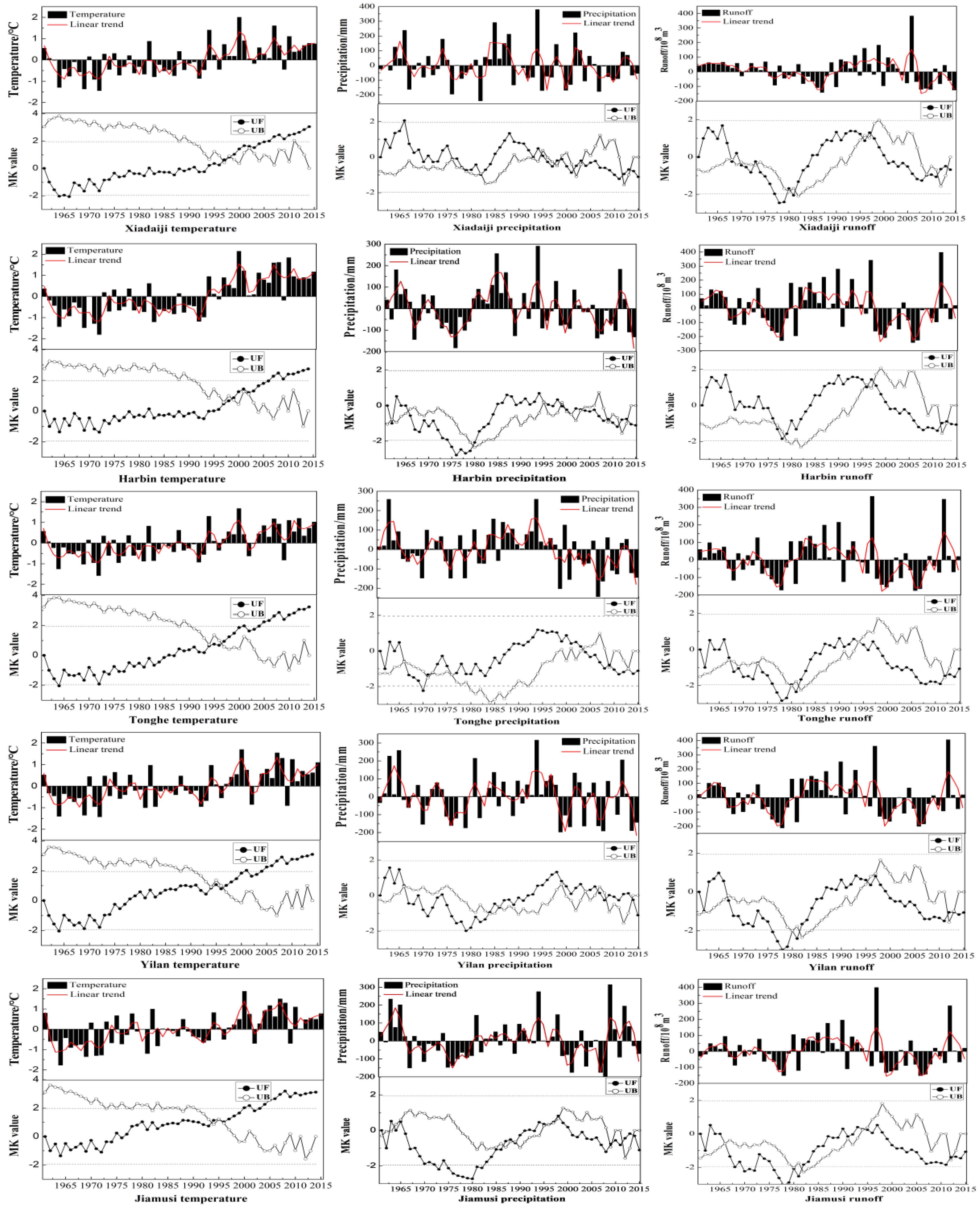
The accuracy scenario simulation was extremely important. The variation trend analysis of temperature and precipitation in the main stream basin of Songhua River during the past 1961–2015 years was combined with the scientific basis for future climate change and put forward in the IPCC reports to reasonably plan for the range of the future temperature and precipitation in the research area.
According to Equation (1), the calibration period of the model extended from 1961 to 2010, and the validation period of the model was from 2010 to 2015. Based on the daily precipitation, temperature and flow data, the model parameters were established in the curve fitting toolbox (cftool) of MATLAB (Matlabsoftware v. 2010b, MathWorks, Natick, Massachusetts, MA, USA). The RSMs of the flood season in the Songhua River basin are shown in Table 3. The coefficient of determination expressed as R2 showed that the simulation results of each region were satisfactory.
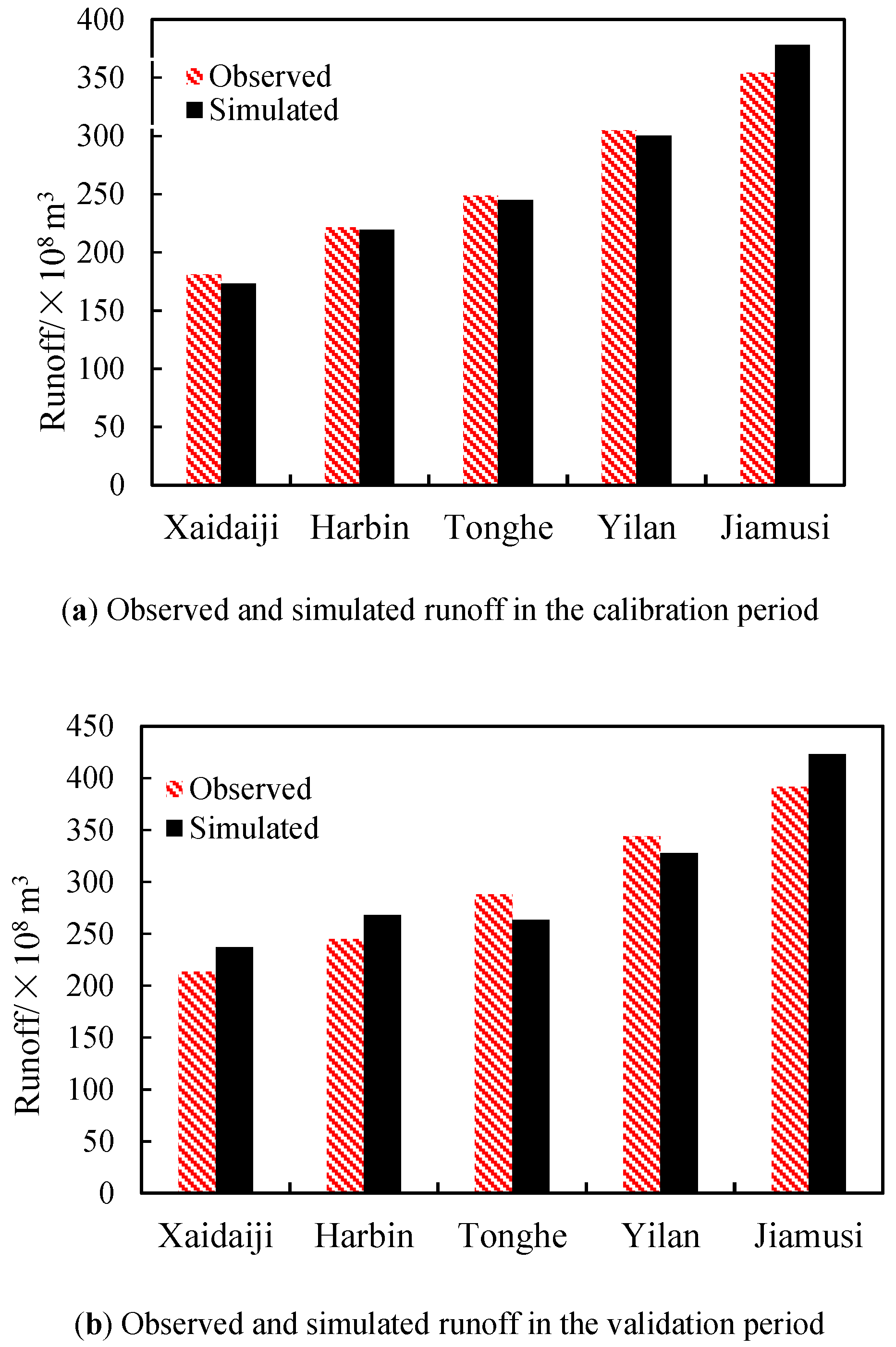
Observed and simulated runoffs in the calibration and validation periods are shown in Figure 4. The REs of Xiadaiji, Harbin, Tonghe, Yilan and Jiamusi between the measured runoff and the simulated runoff in the calibration period were 1.15–34.07%, 1.05–36.71%, 0.69–22.4%, 1.33–35.89%, and 0.45–22.08%, respectively, and those in the validation period were 4.77–26.34%, 4.07–32.45%, 3.75–20.70%, 2.05–11.30%, and 3.50–19.31%, respectively. The CCs of Xiadaiji, Harbin, Tonghe, Yilan and Jiamusi between measured runoff and simulated runoff in the calibration period were 0.874, 0.927, 0.849, 0.862, and 0.810, respectively, and those during the validation period were 0.891, 0.869, 0.725, 0.803, and 0.687, respectively. The RE and CC results suggest that the fitting effects of the runoff simulation models in the five regions were satisfactory, and the RSM can accurately predict runoff in different scenarios.
Assuming that the changes in temperature and precipitation were independent of other climatic factors, various temperature and precipitation scenarios were established for the study area using the random scenarios method [39]. Scenario analysis was adopted in this paper to comprehensively determine the annual trends in temperature and precipitation based on IPCC reports and the analysis of Figure 3. The temperature range was set to −0.5–2 °C, and the range of precipitation varied from −35–30% of the average precipitation from 1961–2015. First, the change in PET in the study area was calculated for the temperature change scenarios. Then, the RSM was used to analyse the rate of runoff change in the future scenarios. Twenty-five scenarios, denoted as S1, S2, S3,…, S25, were analysed (Table 4).
As shown in Table 4, as the temperature in the Songhua River basin increased, the runoff estimated by the RSM decreased, and the runoff increased with a decreasing temperature. As precipitation in the Songhua River basin increased, the runoff predicted by the RSM increased, and the runoff decreased with a decreasing precipitation. Two extremes can be observed in Table 4. First, when the temperature increased by 2 °C and the precipitation decreased by 35%, the simulated runoff decreased by 36.76% compared to the average annual runoff. Second, when the temperature decreased by 0.5 °C and the precipitation increased by 30%, the simulated runoff increased by 30.74% compared to the average annual runoff. These two scenarios reflected extreme drought and extreme flooding, respectively. Additionally, when the temperature and precipitation remain unchanged, the runoff simulated by RSM differs from the measured runoff by 1.03%. This finding further verified the fitting effects of the models, which can be used to optimally allocate water resources.

3.3. Model Parameter Calibration

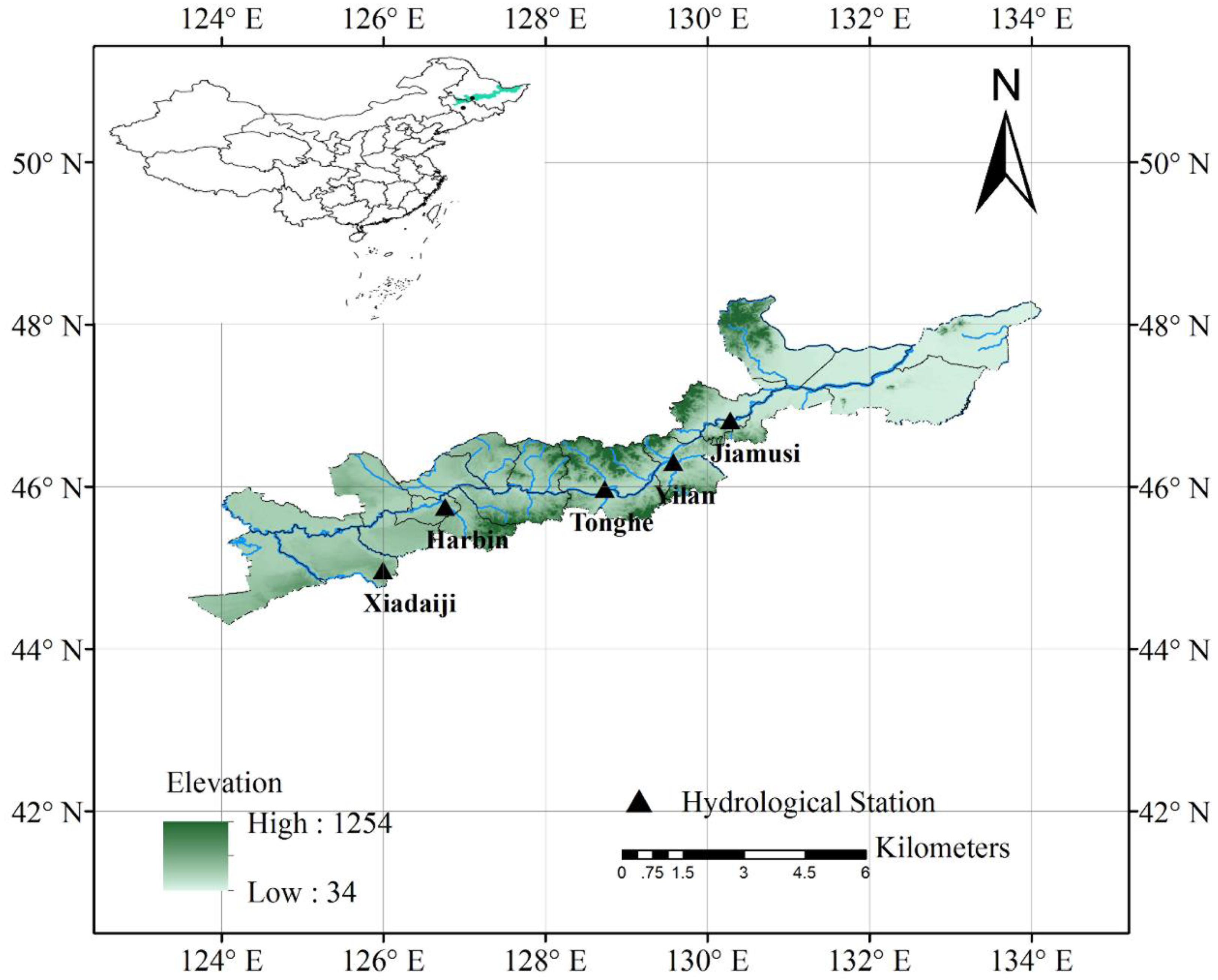
In this paper, the SLFP model is used to maximize improved the proportion of production based on the available water resources inputs. The main stream of the Songhua River is divided into eight subregions according to their associated administrative regions, thus, i = 8 in the model. The water allocation regions were Qianguo, Fuyu, Zhaoyuan, Zhaodong, Harbin (urban area including Shuangcheng, Hulan, Acheng, Bin, Bayan, Mulan, Tonghe, Fangzheng, and Yilan), Jiamusi (urban area including Tangyuan, Huachuan, Fujin, and Tongjiang), Luobei, and Suibin. Sequentially the subregions were numbered: P1, P2, …, P8.
Table 5 shows the added value per unit of water resources and the number of people supplied in different sectors during the two planning periods. To facilitate the calculations, the production value was introduced into the paper. We defined the production value as the value produced in different industries using water. Table 6 shows the other parameters used in the model.

3.4. Water Resource Optimization

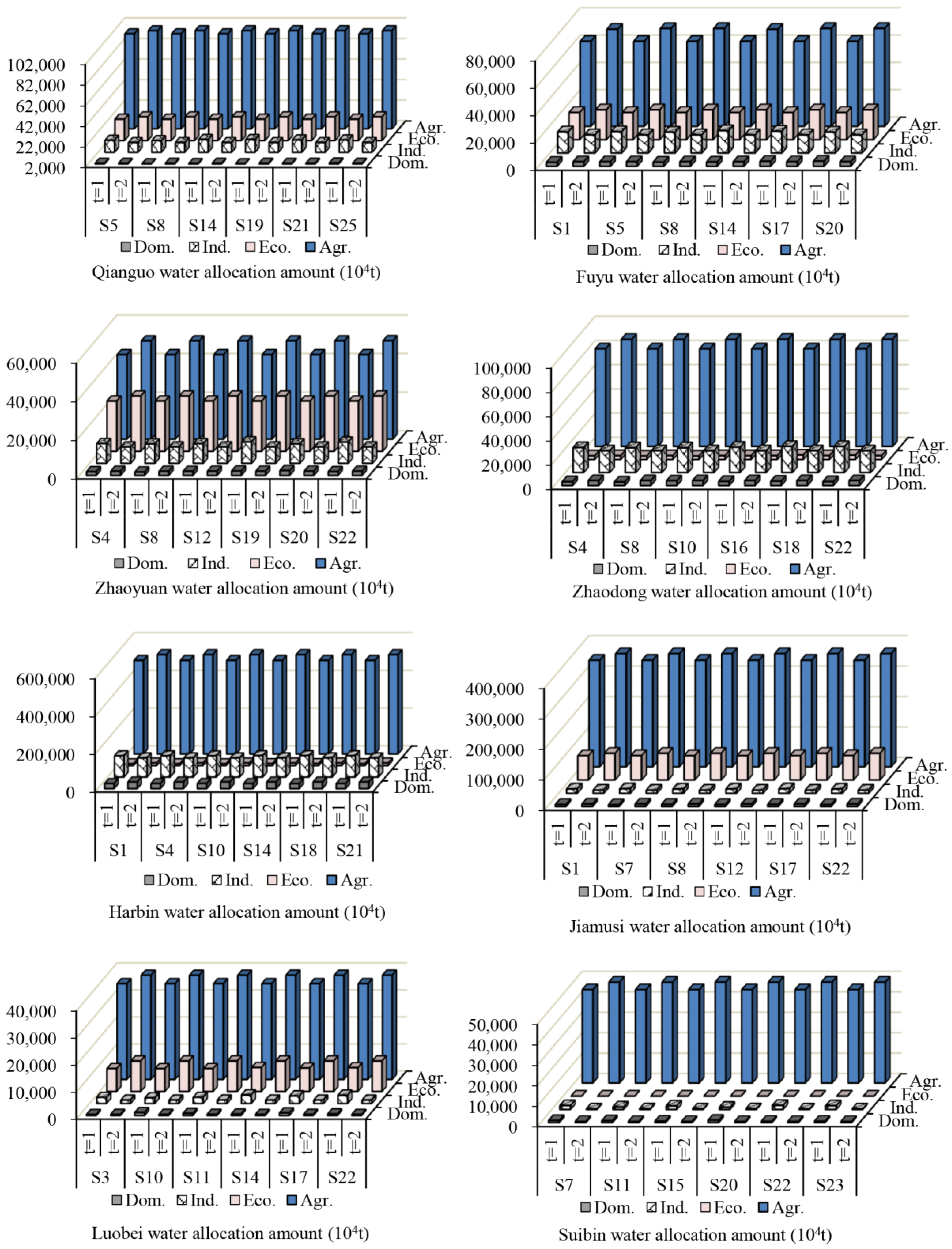
Figure 5 showed the results of the SLFP model. Six typical water allocation schemes are established in each region, and the allocation of water resources varied in each scenario. By assessing the allocation of water resources, the values of water resources and water inputs, as well as the associated trends, can be determined.
A reasonable water allocation scheme can improve economic and social development, as well as improve people’s material and cultural life. Figure 5 shows the water allocation in different periods in each region based on 25 scenarios. Comparing the water allocation of domestic water in different target years, it is found that the trend of water allocation varies in different regions. Due to the large population density and population growth trend, the water allocation in 2030 is higher than 2020, and the water allocation increased by 0.05%, 0.44%, 1.01% and 0.20% in Qianguo, Zhaodong, Harbin and Jiamusi, respectively. Because of the sparse population density, the population has a negative growth trend, the water allocation in 2030 is less than the water allocation in 2020, and the water allocation is reduced by 0.22%, 0.14%, 0.72% and 0.69% in Fuyu, Zhaoyuan, Luobei and Suibin, respectively. The industrial sector, as a water user with the largest actual economic benefit per cubic meter of water, is proportional to the economic and environmental pollution, so the constraint conditions are introduced to restrict the water allocation in the industrial sector to ensure the fairness of the other three water use sectors. The industrial water allocation in 2030 was significantly lower than that in 2020, Qianguo, Fuyu, Zhaoyuan, Zhaodong, Harbin, Jiamusi, Luobei, and Suibin decreased by 2.06%, 3.45%, 3.26%, 3.52%, 2.49%, 1.03%, 3.06% and 2.77% respectively. This is also closely related to the improvement of industrial production water-saving technology and the adjustment of industrial structure. As the largest user of water in four water demand sectors, the water demand of agriculture accounts for the largest proportion of the total water supply. The proportion of agricultural water supply varies in different regions due to planting area, planting species and wetland holdings. The agricultural water supply accounts for 70.92%, 63.27%, 54.79%, 76.21%, 77.22%, 77.68%, 74.76% and 96.59% of the total water supply in Qianguo, Fuyu, Zhaoyuan, Zhaodong, Harbin, Jiamusi, Luobei, and Suibin, respectively. The environmental water allocation in 2030 was projected to be higher than that in 2020 in different regions. The growth rate of environmental water allocation is 1.29%, 0.22%, 0.12%, 0.19%, 0.45%, 0.64% and 3.74% in Qianguo, Fuyu, Zhaoyuan, Zhaodong, Harbin, Jiamusi, Luobei, and Suibin, respectively. Additionally, the population’s awareness of environmental protection is expected to gradually increase; therefore, providing adequate water for environmental uses is important.
Table 7 compared the coefficients of variation for each region and in different periods for different water demand sectors with the 25 scenarios. Notably, in 2020, the water allocation in different sectors was affected by different scenarios, and the fluctuation in 2030 was smaller. In 2020, the domestic water allocation in Luobei was most affected by these different scenarios, while Harbin was the least affected by the different scenarios. The coefficient of variation of the industrial water allocation was largest in Suibin and smallest in Harbin. The coefficient of variation of the environmental water allocation was largest in Zhaodong. Because of the large amount of agricultural water, the difference in agricultural water allocation in different situations is not obvious, which leads to the smaller T, but it can still be seen that the change in water allocation in different scenarios in 2020 is more obvious than that in 2030.
When the objective function is only considered Equation (12), in which only the largest economic benefit is taken into account. The results show that the water allocation for industrial is higher, the water allocation for agricultural is low, the water allocation for ecological changes little, and the water allocation for domestic is basically the same. When the objective function is only considered Equation (16), in which only the minimum water supply target is considered, The results show that water allocation only satisfies the minimum water requirement of each section. When these two target functions were taken into consideration at the same time, the results of water allocation tend to be the result of the target with the minimum water supply. However, consider with Equation (12) limited, it is different from the water allocation results that only consider Equation (16). Because this paper uses fractional linear programming to indirectly represent multiple targets, the two targets are integrated into one model, instead of using traditional weights or only goal programming. In addition to the indirect reflection of two objectives, the model is more important to reflect the efficiency of the system. Because of the shortage of water resources, the decision-makers pay more attention to the efficiency of the allocation, while the fractional linear programming reflects the allocation efficiency index in the form of objective function in the optimization model primarily, so as to efficiently allocate the water resources in the study area.
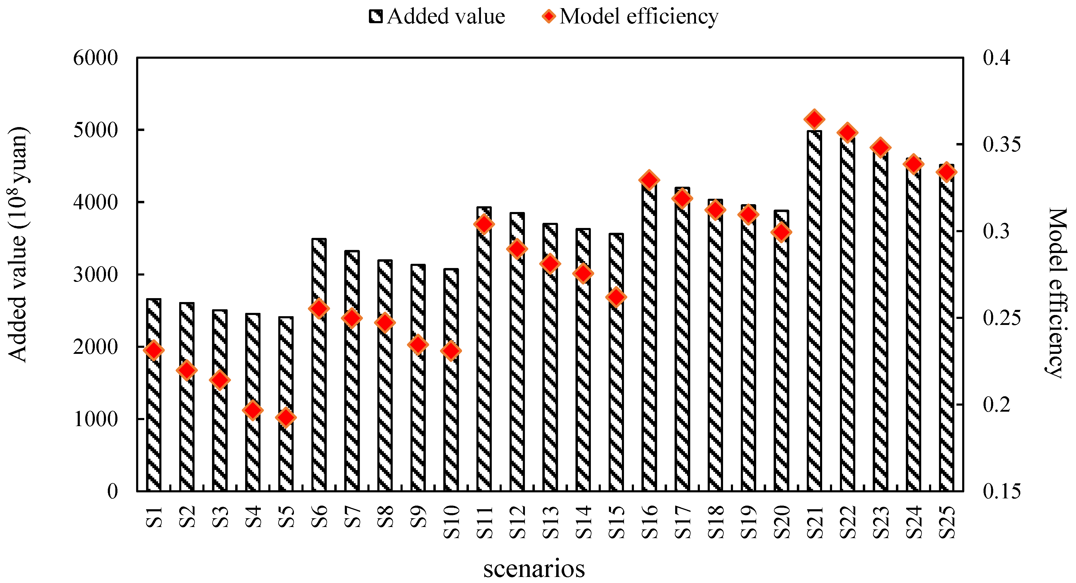
Figure 6 shows the added value and model efficiency under different scenarios. Notably, the higher the runoff, the larger the added value and model efficiency. For example, the added value was 498.09 billion and the model efficiency was 0.365 for S21, which is associated with the largest amount of runoff. The model efficiency of different scenarios reflected the relationships between system benefits and runoff. The system efficiency will increase as runoff increases. Specifically, the higher the amount of runoff, the larger the potential system benefits and economic results. Thus, larger system benefits were produced by relatively large water resources investments, but overly large water supplies can cause natural disasters, such as floods. Moreover, the lower the amount of runoff, the smaller the system benefits, but too little water can also cause natural disasters, such as droughts. As shown in Figure 6, S5 and S21 represented extreme droughts and extreme floods, respectively. The air temperature was increased by 2 °C, and the precipitation was 65% of the annual average precipitation, and the simulated runoff was 63.24% of the annual average runoff in S5. The most needed water sectors should be supplied. At this time, the water conservancy project plays a major role, and we can obtain water from the reservoir and the water diversion project so that society can function normally. The air temperature was decreased by 0.5 °C, and the precipitation was 130% of the annual average precipitation, and the simulated runoff was 130.74% of the annual average runoff in S21. In order not to cause a large area of flood disaster, in addition to provide normal life and the necessary water requirements, the remaining water can also be stored in the reservoir or discharged into the sea through the water diversion project. Thus, it is important to undertake water conservancy projects.
In this paper, we used two types of software to calculate the constructed model: one is Lingo and the other is Excel programming solution. The Lingo model use dual theory, which transforms the fractional programming model into a conventional linear programming model, and Excel uses generalized reduced gradient (GRG) algorithms. Compared with the results of two software solutions, the allocation results are different from the numerical value, but there is not much difference. It is proved that the two types of software are applicable to the solution of the model.
The real-world case study showed that the SLFP model, which considers the changes of temperature and precipitation, is an effective tool for optimally allocating water resources under different water inflow conditions. Generally, compared with other optimization methods, the SLFP model has the following advantages. (i) The SLFP model considers issues such as climate change in a traditional model of optimal water resource allocation to improve the temporal applicability and practicality of the method. Moreover, the model coordinates the relationship between the maximum economic benefits, minimum water supply and maximum water resource efficiency to provide a reference for water resource allocation under different water conditions; (ii) The SLFP model is particularly sensitive to water supply, water requirement, and water allocation constraints. In the modelling process, constraints are carefully established according to COD, water supply, structural adjustments and future national happiness requirements. These constraints can improve the industrial structure. The real-world case study yielded a series of optimal Pareto solutions, and these solutions indicated that all the constraint conditions contributed to the final optimization results; (iii) The SLFP model can provide sufficient analysis of the interrelationships among system efficiency, the investment in water resources and economic benefits. The best effect of the model was observed after long-term use. Therefore, the SLFP method can be applied to other resources, such as reservoir operation management, sustainable waste management, etc.

4. Conclusions

In this study, runoff in the study area was simulated and forecasted considering the future variations of annual precipitation and temperature according to IPCC reports and Figure 3, based on which, a SLFP model for water resources optimal allocation was developed by incorporating the RSM model and LFP model. Through solving the SLFP model, various optimal allocation schemes of water resources in different periods and different scenarios were obtained. The main conclusions can be drawn:
(a)
Based on the Mann-Kendall test of hydro-meteorological data from 1961 to 2015 for the Songhua River basin, the average temperature increased by 0.0278 °C per year, and precipitation presented large fluctuations, while the overall trends of runoff changed slightly. Based on the IPCC reports, 25 scenarios were established considering the variations in temperature and precipitation. The rate of simulated runoff change was 0.0103 with the temperature and precipitation unchanged. The reliability of the RSM was verified by RE and CC. The R2 values of the RSM models were all above 0.81, indicating that the RSM model can provide reliable forecasting and thus can be used as an input of water resource planning.
(b)
The water allocation schemes were affected by different scenarios, and the range of water allocation considerably varied among different regions and sectors in 2020. However, the water allocation was gradually optimized using the SLFP model, and the range of water allocation in different regions and sectors generally decreased in 2030 compared to that in 2020. According to the analysis of the results of water allocation, the economic benefits have been obtained in target years. In this paper, the environmental oxygen demand (EcCOD) and the happy life index were integrated into the SLFP model to improve its practicability. Analysis results of the water resource allocation schemes under the two extreme scenarios indicate that the water resource allocation in the main stream basin of the Songhua River needs water conservancy projects. Using the SLFP model, managers can easily and optimally allocate water resources under different water inflow conditions.

Author Contributions

Q.F. and M.L. designed the study. L.L. wrote the manuscript. T.L. performed the data analysis. S.C. and D.L. reviewed and approved the manuscript.

Funding

This research was funded by the National Key R&D Plan (2017YFC0406002) and the National Natural Science Foundation of China (51709044 and 51479032).

Acknowledgments

The authors acknowledge data support from “National Earth System Science Data Sharing Infrastructure, National Science & Technology Infrastructure of China (http://www.geodata.cn)”.

Conflicts of Interest

The authors declare no conflicts of interest.

References

  1. Pierre, C.; Bernard, P.; Wilson, S.; Thomas, C. Climate change threats to environment in the tropical Andes: Glaciers and water resources. Reg. Environ. Chang. 2011, 11, 179–187. [Google Scholar]
  2. Cheng, K.; Fu, Q. Adaptive allocation modeling for a complex system of regional water and land resources based on information entropy and its application. Water Resour. Manag. 2015, 29, 4977–4993. [Google Scholar] [CrossRef]
  3. Fu, Q.; Li, T.X. Simulation study of the sustainable utilization of urban water resources based on system dynamics: A case study of Jiamusi. Water Sci. Technol. Water Supply 2016, 16, 980–991. [Google Scholar]
  4. Nicklow, J.; Reed, P.; Savic, D.; Dessalegne, T.; Harrell, L.; Chan-Hilton, A.; Karamouz, M.; Minsker, B.; Ostfeld, A.; Singh, A.; et al. State of the art for genetic algorithms and beyond in water resource planning and management. J. Water Resour. Plan. Manag. 2010, 136, 412–432. [Google Scholar] [CrossRef]
  5. Huang, G.H.; Loucks, D.P. An inexact two-stage stochastic programming model for water resources management under uncertainty. Civ. Eng. Environ. Syst. 2000, 17, 95–118. [Google Scholar] [CrossRef]
  6. Lv, Y. Planning regional water resources system using an interval fuzzy bi-level programming method. J. Environ. Inform. 2010, 16, 43–56. [Google Scholar] [CrossRef]
  7. Tabari, M.M.R.; Soltani, J. Multi-objective optimal model for conjunctive use management using SGAs and NSGA-II models. Water Resour. Manag. 2013, 27, 37–53. [Google Scholar] [CrossRef]
  8. Brouwer, M.A.; van den Bergh, P.J.; Aengevaeren, W.R.; Veen, G.; Luijten, H.E.; Hertzberger, D.P.; van Boven, A.J.; Vromans, R.P.; Uijen, G.J.; Verheugt, F.W. Use of multi-objective particle swarm optimization in water resources management. J. Water Resour. Plan. Manag. 2008, 134, 257–265. [Google Scholar]
  9. Higgins, A.; Archer, A.; Hajkowicz, S. A stochastic non-linear programming model for a multi-period water resource allocation with multiple objectives. Water Resour. Manag. 2008, 22, 1445–1460. [Google Scholar] [CrossRef]
  10. Zhang, C.; Guo, P. A generalized fuzzy credibility-constrained linear fractional programming approach for optimal irrigation water allocation under uncertainty. J. Hydrol. 2017, 553, 735–749. [Google Scholar] [CrossRef]
  11. Mani, A.; Tsai, T.C.; Paudel, K.P. Mixed integer linear fractional programming for conjunctive use of surface water and groundwater. J. Water Resour. Plan. Manag. 2016, 142, 04016045. [Google Scholar] [CrossRef]
  12. Ren, C.F.; Guo, P.; Li, M.; Gu, J.J. Optimization of industrial structure considering the uncertainty of water resources. Water Resour. Manag. 2013, 27, 3885–3898. [Google Scholar] [CrossRef]
  13. Field, C.B.; Barros, V.R.; Mach, K.; Mastrandrea, M. Climate Change 2014: Impacts, Adaptation, and Vulnerability; Contribution of Working Group II to the Third Assessment Report; World Meteorological Organization: Geneva, Switzerland, 2014; Volume 19, pp. 81–111. [Google Scholar]
  14. Flato, G.; Marotzke, J.; Abiodun, B.; Braconnot, P.; Chou, S.C.; Collins, W.J.; Cox, P.; Driouech, F.; Emori, S.; Eyring, V.; et al. Evaluation of Climate Models. In Climate Change 2013: The Physical Science Basis; Contribution of Working Group I to the Fifth Assessment Report of the Intergovernmental Panel on Climate Change; IPCC: Geneva, Switzerland, 2013; Volume 18, pp. 95–123. [Google Scholar]
  15. Orr, H. Climate change in Contrasting River Basins: Adaptation Strategies for Water, Food and Environment. Geogr. J. 2006, 172, 352–353. [Google Scholar] [CrossRef]
  16. Taylor, K.E.; Stouffer, R.J.; Meehl, G.A. An overview of CMIPS and the experiment design. Bull. Am. Meteorol. Soc. 2012, 93, 485–498. [Google Scholar] [CrossRef]
  17. Chen, H.P. Projected change in extreme rainfall events in China by the end of the 21st century using CMIP5 models. Chin. Sci. Bull. 2013, 58, 1462–1472. [Google Scholar] [CrossRef]
  18. Li, L.; Li, W.; Deng, Y. Summer rainfall variability over the Southeastern United States and its intensification in the 21st century as assessed by CMIP5 models. J. Geophys. Res. Atmos. 2013, 118, 340–354. [Google Scholar] [CrossRef]
  19. Guo, Y.; Dong, W.; Ren, F. Assessment of CMIP5 simulations for China annual average surface temperature and its comparison with CMIP3 simulations. Progress. Inquis. Mutat. Clim. 2013, 9, 181–186. [Google Scholar]
  20. O’Neill, B.C.; Oppenheimer, M.; Warren, R.; Hallegatte, S.; Kopp, R.E.; Pörtner, H.O.; Scholes, R.; Birkmann, J.; Foden, W.; Licker, R. IPCC reasons for concern regarding climate change risks. Nat. Clim. Chang. 2017, 7, 28–37. [Google Scholar] [CrossRef]
  21. Zhang, S.F.; Hua, D.; Meng, X.J.; Zhang, Y.Y. Climate change and its driving effect on the runoff in the “Three-River Headwaters” Region. Acta Geogr. Sin. 2011, 21, 963–978. [Google Scholar] [CrossRef]
  22. Najafi, M.R.; Moradkhani, H. A hierarchical bayesian approach for the analysis of climate change impact on runoff extremes. Hydrol. Process. 2015, 28, 6292–6308. [Google Scholar] [CrossRef]
  23. Jiang, T.; Chen, Y.D.; Xu, C.Y.; Chen, X.; Chen, X.; Vijay, P.S. Comparison of hydrological impacts of climate change simulated by six hydrological models in the Dongjiang Basin, South China. J. Hydrol. 2007, 336, 316–333. [Google Scholar] [CrossRef]
  24. Milly, P.C.D.; Betancourt, J.; Falkenmark, M.; Hirsch, R.M.; Kundzewicz, Z.W.; Lettenmaier, D.P.; Stouffer, R.J. Stationarity is dead: Whither water management? Science 2008, 319, 573–574. [Google Scholar]
  25. Nourani, V.; Kisi, O.; Komasi, M. Two hybrid artificial intelligence approaches for modeling rainfall—Runoff process. J. Hydrol. 2011, 402, 41–59. [Google Scholar] [CrossRef]
  26. Liu, C.M. The Impact of Climatic Change on the Hydrological Situation of China; China Meteorological Press: Beijing, China, 1993. [Google Scholar]
  27. Yu, F.; Zhang, G.H.; Liu, Y.M. Analysis on effects of global climate change on water resource in the Yellow River Basin. J. China Hydrol. 2008, 28, 52–56. [Google Scholar]
  28. Makkink, G.F. Testing the penman formula by means of lysimeters. J. Inst. Water Eng. 1957, 11, 277–288. [Google Scholar]
  29. Pristley, C.H.B.; Taylor, R.J. On the assessment of surface heat flux and evaporation using large-scale parameters. Mon. Weather Rev. 2009, 100, 81–92. [Google Scholar] [CrossRef]
  30. Abtew, W. Evapotranspiration measurement and modeling for three wetland systems in South Florida. J. Am. Water Resour. Assoc. 1996, 32, 465–473. [Google Scholar] [CrossRef]
  31. Hargreaves, G.H. Moisture Availability and Crop Production; American Society of Agricultural and Biological Engineers: St. Joseph, MI, USA, 1975; Volume 18, pp. 980–984. [Google Scholar]
  32. Doorenbos, J.; Pruitt, W.O. Guidelines for Predicting Crop Water Requirements; FAO Irrigation and Drainage Paper; FAO: Rome, Italy, 1975. [Google Scholar]
  33. Penman, H.L. Natural evaporation from open water, bare soil, and grass. Proc. R. Soc. A 1948, 193, 120. [Google Scholar] [CrossRef]
  34. Neitsch, S.; Arnold, J.; Kiniry, J.; Williams, J. Soil and Water Assessment Tool: Theoretical Documentation; Agricultural Research Service: Temple, TX, USA, 2002.
  35. Thomas, A. Spatial and temporal characteristics of potential evapotranspiration trends over China. Int. J. Climatol. 2015, 20, 381–396. [Google Scholar] [CrossRef]
  36. Zhang, Y.F.; Deng, J.L.; Guan, D.X. Spatiotemporal changes of potential evapotranspiration in Songnen Plain of Northeast China. Chin. J. Appl. Ecol. 2011, 22, 1702–1710. [Google Scholar]
  37. Li, M.; Guo, P.; Liu, X.; Huo, G.H.Z. A decision-support system for cropland irrigation water management and agricultural non-point sources pollution control. Desalination Water Treat. 2014, 52, 5106–5117. [Google Scholar] [CrossRef]
  38. Chadha, S.S.; Chadha, V. Linear fractional programming and duality. Cent. Eu. J. Oper. Res. 2007, 15, 119–125. [Google Scholar] [CrossRef]
  39. Smith, J.W.; Dugan, R.; Rylander, M. Advanced distribution planning tools for high penetrate-on PV deployment. In Proceedings of the Power and Energy Society General Meeting, San Diego, CA, USA, 22–26 July 2012; pp. 1–7. [Google Scholar]
Figure 1. Geographical location of the study area and the locations of hydrological stations.
Water 10 00627 g001
Figure 2. Decision procedure of the developed framework for water resource planning.
Water 10 00627 g002
Figure 3. Variations and Manner-Kendall-Sneyers trend test of temperature, precipitation and runoff in the main stream of the Songhua River.
Water 10 00627 g003
Figure 4. Observed and simulated runoff in the calibration and validation periods.
Water 10 00627 g004
Figure 5. Water allocation in different regions of the study area. Note: Dom. refers to domestic water allocation amount; Ind. refers to industrial water allocation amount; Eco. refers to environmental water allocation amount; Agr. refers to agricultural water allocation amount.
Water 10 00627 g005
Figure 6. Added value and model efficiency under different scenarios.
Water 10 00627 g006
Table 1. The average air temperature, precipitation and solar radiation during the flood season at five meteorological stations in the study area from 1961–2015.
StationCodeLatitudeLongitudeTemperature (°C)Precipitation (mm)Solar Radiation (MJ m−2 day−1)
Xiadaiji5406344°58′126°00′20.40387.24217.27
Harbin5095345°45′126°26′19.94419.84205.37
Tonghe5096345°58′128°44′18.80397.52207.92
Yilan5087746°18′129°35′18.97401.37197.22
Jaimusi5087346°49′130°17′19.18381.59197.16
Table 2. Model parameter.
ParameterDescriptionUnits
DoWSitthe water supply for domestic use in area i and period tm3
InWSitthe water supply for industry in area i and period tm3
AgWSitthe water supply for agriculture in area i and period tm3
EcWSitthe water supply for the environment and wetlands in area i and period tm3
InVitthe industrial value added per unit of water supply in area i and period tyuan/m3
AgVitthe agricultural value added per unit of water supply in area i and period tyuan/m3
EcVitthe environmental and wetland value added per unit of water supply in area i and period tyuan/m3
WSPitthe number of people supported per unit of water supply in area i and period tp/m3
CCEitthe per capita consumption expenditure in area i and period tyuan/p
DSOCtthe operating costs of sewage treatment plants per unit of domestic sewage in period t, t1 requires 0.53 yuan/m3, and t2 requires 0.50 yuan/m3yuan/m3
IWOCtthe operating costs of sewage treatment plants per unit of industrial wastewater in period t, t1 requires 3.18 yuan/m3, and t2 requires 3.06 yuan/m3yuan/m3
DSTRtthe rate of domestic sewage treatment in period t, t1 requires 0.9018, and t2 requires 0.9547-
IWTRtthe rate of industrial wastewater treatment in period t, t1 requires 0.9532, and t2 requires 0.9918-
DSDtthe per capita domestic sewage discharge in period tm3/p
IWDtthe industrial wastewater discharge per unit GDP in period tm3/yuan
DoCODtthe COD discharge of domestic pollution sources per capita in period tm3/p
InCODtthe COD discharge of industrial pollution sources per unit GDP in period tm3/yuan
AgCODtthe COD discharge of agricultural pollution sources per unit GDP in period tm3/yuan
RSTCODtthe rate of COD disposal in sewage treatment plants in period t, t1 requires 0.9245, and t2 requires 0.9538-
OCDCODtthe operating costs of sewage treatment plants per unit of COD discharge from domestic pollution sources in period tyuan/p
OCICODtthe operating costs of sewage treatment plants per unit of COD discharge from industrial pollution sources in period tyuan/m3
OCACODtthe operating costs of sewage treatment plants per unit of COD discharge from agricultural pollution sources in period tyuan/m3
EcCODtthe environmental capacity of CODs in a certain environmental scope in period tm3
R0ithe runoff simulated by RSM in area im3
WURtthe utilization ratio of surface water resources in period t, t1 requires 0.5, and t2 requires 0.85-
MinDoWSitthe minimum water supply for domestic use in area i and period tm3
MinInWSitthe minimum water supply for industry in area i and period tm3
MinAgWSitthe minimum water supply for agriculture in area i and period tm3
MinEcWSitthe minimum water supply for the environment and wetlands in area i and period tm3
Note: p refers to population.
Table 3. Runoff simulation model in different regions during the flood season.
RegionRunoff Simulation ModelR2
XiadaiijiR0 = 686.7811P0.8988ET−0.9083R2 = 0.8512
HarbinR0 = 871.9465P0.9138ET−0.9225R2 = 0.8162
TongheR0 = 1674.5940P0.8880ET−0.9911R2 = 0.8572
YilanR0 = 1619.9227P0.9272ET−0.9862R2 = 0.8647
JiamusiR0 = 2105.5688P0.8966ET−0.9588R2 = 0.8110
Table 4. The rate of runoff change during the flood season in the study area under future scenarios.
TT − 0.5 °CTT + 1°CT + 1.5 °CT + 2 °C
P
P × (1 − 35%)−30.20−31.59−34.26−35.53−36.76
P × (1 − 15%)−11.01−12.79−16.19−17.81−19.38
P3.091.03−2.90−4.78−6.60
P × (1 + 10%)12.3910.145.853.801.81
P × (1 + 30%)30.7428.1223.1320.7518.44
Note: T refers to temperature; P refers to precipitation.
Table 5. The added value of the industrial, agricultural, and environmental sectors per unit of water resources produced relative to the water supply to the population.
RegionsInV (yuan/m3)AgV (yuan/m3)EcV (yuan/m3)WSP (p/m3)
t = 1t = 2t = 1t = 2t = 1t = 2t = 1t = 2
P1107.970157.24515.42819.11720.92922.8320.2540.215
P2102.474149.24125.59631.65320.92922.8320.2440.213
P393.826136.64620.93525.63720.92922.8320.2670.217
P4121.369176.75924.26629.667110.803120.8760.3060.221
P5128.286186.8327.4009.082110.803120.8760.2910.219
P6115.826168.6873.4084.19762.78868.4960.2850.219
P799.470144.8665.4436.71262.78868.4960.2320.211
P894.274137.2984.8986.031000.3260.223
Table 6. Other input parameters.
Target years DSD (m3/p)IWD (m3/yuan)DoCOD (m3/p)InCOD (m3/yuan)AgCOD (m3/yuan)OCDCOD (yuan)OCICOD (yuan)OCACOD (yuan)EcCOD (m3)
t = 128.0830.00070.01986.7 × 10−70.000012422133012618,560
t = 230.1970.000540.01895.9 × 10−70.000009409128912214,848
Table 7. The coefficient of variation for water allocation under different scenarios.
RegionsDomestic Water SectorIndustrial Water SectorEnvironmental Water SectorAgricultural Water Sector
t = 1t = 2t = 1t = 2t = 1t = 2t = 1t = 2
P17.24%0.48%2.23%0.05%0.01%00.14%0.03%
P27.35%0.14%2.69%0.05%4.62%00.12%0.06%
P310.12%0.25%4.39%0.10%0.01%00.10%0.03%
P46.38%0.18%1.51%0.03%8.37%0.09%0.21%0.05%
P51.13%0.06%0.33%0.01%3.24%0.04%0.05%0.03%
P64.16%0.07%2.55%0.06%0.19%0.01%0.09%0.01%
P728.79%1.93%16.27%0.43%0.94%0.02%0.11%0.02%
P821.41%0.82%20.83%2.81%--0.12%0.03%

