Data Pre-Analysis and Ensemble of Various Artificial Neural Networks for Monthly Streamflow Forecasting

1
School of Hydropower and Information Engineering, Huazhong University of Science and Technology, Wuhan 430074, China
2
Hubei Key Laboratory of Digital Valley Science and Technology, Wuhan 430074, China
*
Authors to whom correspondence should be addressed.
Water 2018, 10(5), 628; https://doi.org/10.3390/w10050628
Submission received: 28 March 2018
/
Revised: 28 April 2018
/
Accepted: 7 May 2018
/
Published: 13 May 2018
(This article belongs to the Special Issue Flood Forecasting Using Machine Learning Methods)
Abstract
:This paper introduces three artificial neural network (ANN) architectures for monthly streamflow forecasting: a radial basis function network, an extreme learning machine, and the Elman network. Three ensemble techniques, a simple average ensemble, a weighted average ensemble, and an ANN-based ensemble, were used to combine the outputs of the individual ANN models. The objective was to highlight the performance of the general regression neural network-based ensemble technique (GNE) through an improvement of monthly streamflow forecasting accuracy. Before the construction of an ANN model, data preanalysis techniques, such as empirical wavelet transform (EWT), were exploited to eliminate the oscillations of the streamflow series. Additionally, a theory of chaos phase space reconstruction was used to select the most relevant and important input variables for forecasting. The proposed GNE ensemble model has been applied for the mean monthly streamflow observation data from the Wudongde hydrological station in the Jinsha River Basin, China. Comparisons and analysis of this study have demonstrated that the denoised streamflow time series was less disordered and unsystematic than was suggested by the original time series according to chaos theory. Thus, EWT can be adopted as an effective data preanalysis technique for the prediction of monthly streamflow. Concurrently, the GNE performed better when compared with other ensemble techniques.
1. Introduction
Streamflow forecasting has been one of the key issues in hydrology in recent decades. Enhancing streamflow forecasting accuracy is of great significance to various aspects of hydrological system such as water allocation, flood control, and disaster relief. In recent decades, numerous methods and hydrological models have been studied to obtain accurate streamflow predictions. These methods can be grouped into two categories: conceptual models and empirical models [1]. Conceptual models, also known as physically based models, are designed to simulate the physical mechanism of hydrological processes [2]. However, because of insufficient data collection both in space and time for conceptual models, these models may not be feasible for streamflow forecasting [3]. On the other hand, empirical models are data-driven models which are built using historical information contained in the hydrological time series as opposed to the physical processes of a certain catchment [4,5,6]. The various empirical models involved in hydrological forecasting predominantly include time series models, machine learning methods, and hybrid methods. Time series models, especially auto-regressive moving average models, have been one of the most popular methodologies for streamflow forecasting over the last decades. However, the results of the previous studies have shown that time series models only provide satisfactory results when the series are either linear or near-linear; they do not perform well with non-linear series [1,7].
As a result of this limitation of time series models, in recent years, various machine learning methods have been applied in the forecasting of non-linear hydrological systems. Among the various machine learning methods, artificial neural networks (ANNs), which include backpropagation neural network (BPNN), radial basis function (RBF) neural network, generalized regression neural network (GRNN), Elman neural network, and multi-layer feed-forward (MLFF) network, are among the most popular techniques for hydrological time series forecasting. Chen et al. [8] applied three different ANN models, namely a MLFF network, a RBF network, and a GRNN, to predict the streamflow, and copula–entropy (CE) was utilized to identify the inputs of the networks. Results showed that the MLFF network with the CE method obtained better results in comparison with traditional linear correlation analysis. Chang et al. [9] successfully introduced BPNN, Elman neural network, and NARX network into the forecasting of one-to six-steps ahead of floodwater storage pond water levels. The results indicated that the proposed NARX model could be beneficial for the control of urban floods. Hosseini-Moghari and Araghinejad [10] utilized the recursive and direct versions of Multi-Layer Perceptron (MLP), RBF and GRNN neural networks for forecasting droughts at short-, mid-, and long-term time scales, respectively. Results showed that the recursive models obtained better results at smaller time scales of the Standard Precipitation Index while the direct models showed better performance at longer time scales.
Numerous successes have been obtained in the applications of ANNs for time series forecasting; rooms exists to improve single ANN method performance. One trend to enhance the performance of ANN models for time series forecasting is to employ data-preprocessing techniques [11,12]. Wang et al. [13] presented a hybrid approach which combined ensemble empirical mode decomposition (EEMD) and artificial neural networks for medium and long-term runoff forecasting. Results of this study indicated that EEMD could enhance forecasting accuracy of medium and long-term runoff time series. Zhu et al. [14] developed signal decomposition techniques, including discrete wavelet transform (DWT) and empirical mode decomposition (EMD), to improve the forecasting accuracy of the support vector machine (SVR) models for monthly streamflow prediction. Results have shown both EMD and DWT can improve the forecasting accuracy of monthly streamflow, while DWT performed better EMD in enhancing the forecasting accuracy of the SVM model. Seo et al. [15] compared and evaluated three hybrid models for forecasting daily river stages: the wavelet package-ANN (WPANN) model, the wavelet package-adaptive neuro-fuzzy inference system (WPANFIS) model, and the wavelet package-SVM (WPSVM) model. The results obtained indicated that the WPANFIS models provided better prediction results than the WPANN and WPSVM models. Although WT- and EMD-based data preprocessing techniques have shown their efficiency in promoting the performance of machine learning forecasting methods, the performance of WT is sensitive to the selection of mother wavelets and EMD is likely to be encountered with the mode mixing problem. The Empirical Wavelet Transform (EWT) proposed by Gilles [16] solves these problems. The efficiency of EWT as a data preanalysis method to improve the forecasting accuracy of machine learning methods has been demonstrated in Hu and Wang [17] and Wang and Hu [18] for mean half-hour wind speed and mean 15 min wind speed forecasting, respectively.
To construct an ANN model for streamflow forecasting, one of the most important steps is to determinate appropriate input vectors. Numerous studies have confirmed and verified the existence of chaotic behavior in hydrological time series as that generated by the underlying stochastic processes, the phase space reconstruction (PSR) method has been utilized as an alternative approach to select relevant and important input variables for ANN models [19]. Guo et al. [20] introduced the PSR method to determine the inputs of the SVR streamflow prediction model to overcome the drawbacks in the empirical judgment within the structure of the forecasting model. Hu et al. [21] investigated the cross-scale chaotic behaviors of the runoff processes in an inland river of central Asia by using the PSR technique and chaos theory. Ouyang et al. [22] successfully introduced the PSR method in the construction of an input matrix for SVR models for forecasting monthly rainfall.
Several papers have studied the employment of a single ANN [23], while other have compared the performance of different ANN architectures. Because an ensemble model often can obtain more accurate results than its constituent components, employing ensemble techniques has become a popular topic in recent years to enhance the generalizability and reliability of ANNs. Ensemble techniques have already been successfully applied to numerous time series predictions such as wind and solar power forecasting [24] as well as heating energy consumption predictions [25]. In this study, the objective was to investigate the efficiency of various ensemble techniques including simple averaging ensemble (SAE), weighted averaging ensemble (WAE), and GRNN-based ensemble (GNE) through the combination of the outputs of various single ANN models. Additionally, to take advantage of both the superior performance of EWT in data preanalysis and the PSR technique in selecting input vectors, the EWT and PSR methods were exploited in the proposed ensemble forecasting models. Mean monthly streamflow observation data from Wudongde hydrological station in Jinsha River Basin, China was used to demonstrate the efficiency of the proposed GNE ensemble model.
2. Methodology
2.1. Artificial Neural Networks
2.1.1. Radial Basis Function Neural Network
Radial basis function neural network is type of multilayer and feed-forward neural network (FNN) [26]. Similar to traditional ANNs, the RBF neural network consists of three layers which include: an input layer which composed of input variables, a hidden layer where the input variables are transformed by a nonlinear function, and a linear output layer which produces the network response. In comparison with the most commonly used sigmoidal functions employed by a FNN, the hidden layer of a RBF neural network uses Gaussian transfer functions as activation functions. The Gaussian activation function can be written as:
where is the input vector with N dimensions, is the center of the ith neuron in the hidden layer, is the width of the Gaussian function, and || || is the Euclidean Norm. The response of the jth node in the output layer can be written as
where is the connecting weight between the ith hidden node and the jth output node.
2.1.2. Extreme Learning Machine
Extreme Learning Machine (ELM) developed by Huang et al. [27] is a new type of single hidden layer feed-forward network (SLFN). Given a set of N samples , , the ELM network with L hidden neurons and activation function g can be referred to as:
where ; , is the weight vector that connects the n input neurons with the ith hidden neuron; is the weight vector that connects the ith hidden neuron with the m output neurons; is the bias.
Equation (3) can be abbreviated as:
where
and H is the output matrix of the hidden layer. The output weights of ELM can be obtained by calculating the least square solution of the following equation:
The least square solution can be given as:
where denotes the Moore-Penrose generalized inverse of H [27].
2.1.3. Elman Neural Network
Elman neural network is a kind of dynamic recurrent neural network [28]. In addition to the input layer, hidden layer, and output layer, an Elman network has a special recurrent layer which connects every input unit to a hidden unit; every hidden unit has a corresponding time delay [9]. The recurrent layer is used to store the output information of the hidden layer within a certain time delay; that information is then used as the input for the hidden layer. Therefore, the outputs of the Elman network depend not only on the preset inputs but also on the previous states of the hidden units [9]. In this study, the Elman network was trained using a gradient descent with momentum; the transfer functions of hidden and output layers were of sigmoid and linear types, respectively.
2.1.4. General Regression Neural Network
The GRNN was first introduced by Specht [29] and was a variation of RBF. Assuming a random vector and the joint continuous probability density function is known, the regression of on x can be given by [29,30]:
where is the conditional expect of the output y given the input vector X. The joint density is usually unknown and can be estimated by the Gaussian kernel estimator:
where , n is the number of observations, d is the dimension of X, and σ is the smoothing parameter.
According to Equations (9) and (10), the general version of GRNN can be obtained as follows:
where is the probability estimate function of .
2.2. Phase Space Reconstruction
To transfer a one-dimension time series into a multi-dimensional phase-space, Packard et al. [31] proposed a PSR method. The PSR method can fully uncover the hidden information of the time series. For a given time series , the key of the PSR method is to find the embedded dimension m and the parameter of time delay τ, such that
where represents the kth phase point of the input vector and represents the kth phase point of the output vector.
In this study, the auto-correction function (ACF) value and Average Mutual Information (AMI) were utilized to determine the time delay ; the Cao method [32] was utilized to determine the embedded dimension m. Generally, the time delay is selected when the ACF first passes through zero value or the AMI arrives at the first minimum [33]. The value of m is determined according to Cao [32], once E1 stops changing when d is greater than some value d0. Subsequently, the minimum embedding dimension is selected as d0 + 1. Readers may refer to Cao [32] for more information about the Cao method.
Only time series with chaotic characteristics can obtain accurate forecasting results using chaotic theories. After the time delay and embedded dimension are determined, the chaotic characteristics of the time series should be confirmed. The most commonly used method is the maximum Lyapunov exponent method. If the maximum Lyapunov exponent of the time series is positive, then the time series shows chaos features. Otherwise, and m needs to be redefined. In this study, the small data sets method proposed by Rosenstein et al. [34] was used to calculate the maximum Lyapunov exponent of a time series.
2.3. Empirical Wavelet Transform
Empirical wavelet transform developed by Gilles [16] is used to decompose the given signal into a collection of amplitude modulated–frequency modulated (AM-FM) signals according to the information contained in the Fourier spectrum of the signal. For a given time series , the decomposition processes using EWT can be described in the following five steps.
Firstly, the Fourier spectrum of the original time series was calculated using Fast Fourier Transform Algorithm;
Secondly, the boundaries were determined by proper segmentation of the Fourier spectrum:
where denotes the frequencies corresponding to the local maxima and .
Thirdly, the empirical wavelets and scaling function were constructed:
where , .
Fourthly, and the approximate and detail coefficients were calculated:
Finally, the original signal was reconstructed to obtain different modes:
Readers may refer to Gilles [16] for more information about EWT.
2.4. Ensemble Techniques
The generalizability and reliability of an ANN model can be often improved by appropriate ensemble techniques. Because the forecasting results of the individual models can vary in different data points, the error of the individual networks can be compensated by combining the outputs [25]. In this study, three kinds of ensemble techniques, namely, SAE, WAE, and GNE, were introduced to combine the outputs of different ANNs and were studied.
2.4.1. Simple Averaging Ensemble
The SAE takes advantage of the concept of the arithmetic mean. Consider an ANN ensemble model with K sub-ANNs, the output of the SAE model can be defined as:
where is the output of the kth sub-ANN and N denotes the length of the data set.
2.4.2. Weighted Averaging Ensemble
In the WAE model, the weighted means of the outputs of the sub-ANNs constructed the ensemble output. The output of the WAE model with K sub-ANNs can be defined as:
where denotes the weight of the kth model at point i and . The specific value of is determined according to the absolute error between the observed values and the simulated values. The weights of different models at different points are variational, and the point with smaller absolute error will be given bigger weight. The weight can be calculated as:
where denotes the absolute error of the kth model at point i.
2.4.3. Artificial Neural Network-Based Ensemble
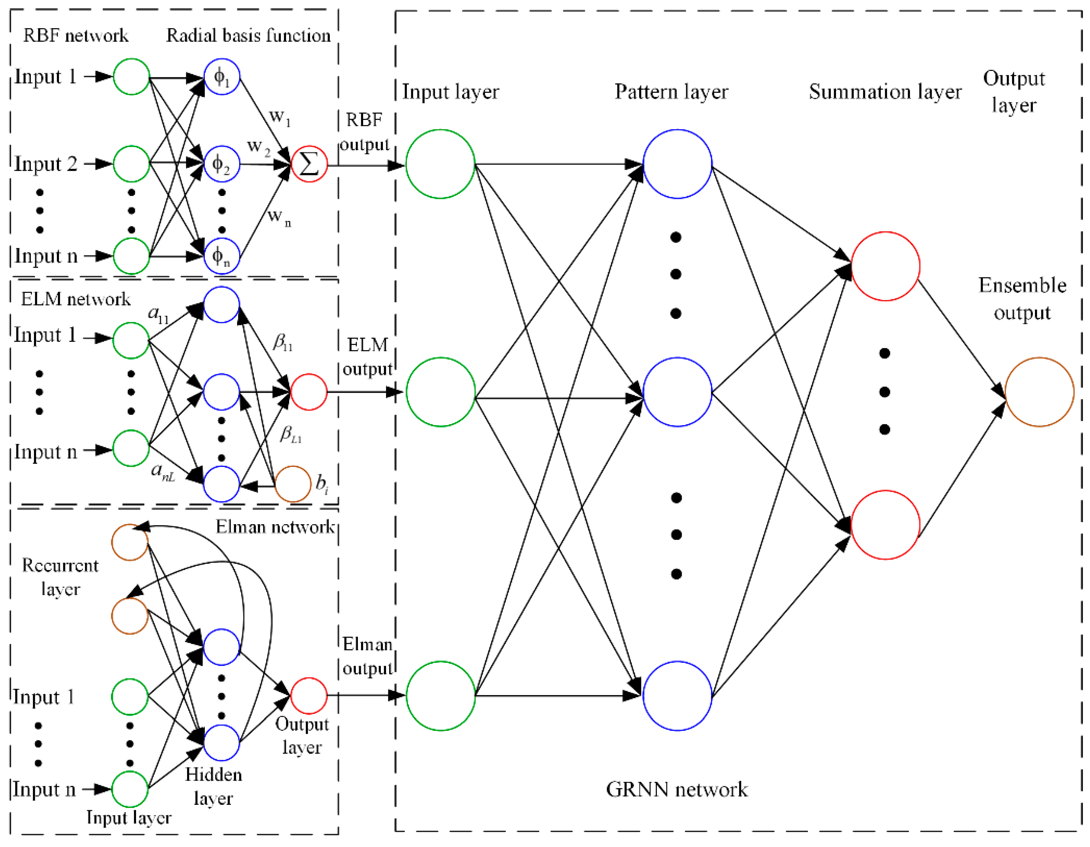
Because the spread of the GRNN model is the only parameter to be optimized, error caused by uncertainty in the parameters can be decreased. Thus, the GRNN network was chosen as the ensemble technique to enhance the performance of the single ANN. In the GNE model, the forecasting results of the RBF, ELM, and Elman networks were taken as input variables, while the target variable was taken as the output variable. The GRNN network was trained to obtain the best model parameter. The forecasting result of the GRNN network was taken as the result of the GNE model. The weight coefficients of the RBF, ELM, and Elman models were variational and the accurate weight of these models could not be obtained because of the black-box principle of the GRNN neural network. The structure of the GRNN ensemble forecasting model, using the RBF, ELM, and Elman models, is shown in Figure 1.
2.5. Model Performance Evaluation
It is important to apply multiple error measure indices when evaluating the forecasting ability of the developed models. Four measures, the root mean square error (RMSE), the mean absolute error (MAE), the mean absolute percent error (MAPE), and the coefficient of correlation (R,) have been used in this paper [35]. Among the four statistical measures, RMSE was sensitive to the extremely large or small values of a time series and reflected the degree of variation, the MAE reflected the actual forecasting error in a more balanced perspective, and the MAPE was a measure of accuracy for the forecasted streamflow series with no units. The RMSE, MAE, and MAPE are defined as:
where and are the predicted and observed monthly streamflow series, respectively, and N is the length of the data.
The R describes the degree to which two data sets are related and ranges from −1 to 1. The larger the absolute value of the correlation coefficient, the more the predicted and observed data is related. The correlation coefficient is defined as:
where and indicate the average value of the predicted and observed runoffs, respectively.
2.6. Modeling Framework
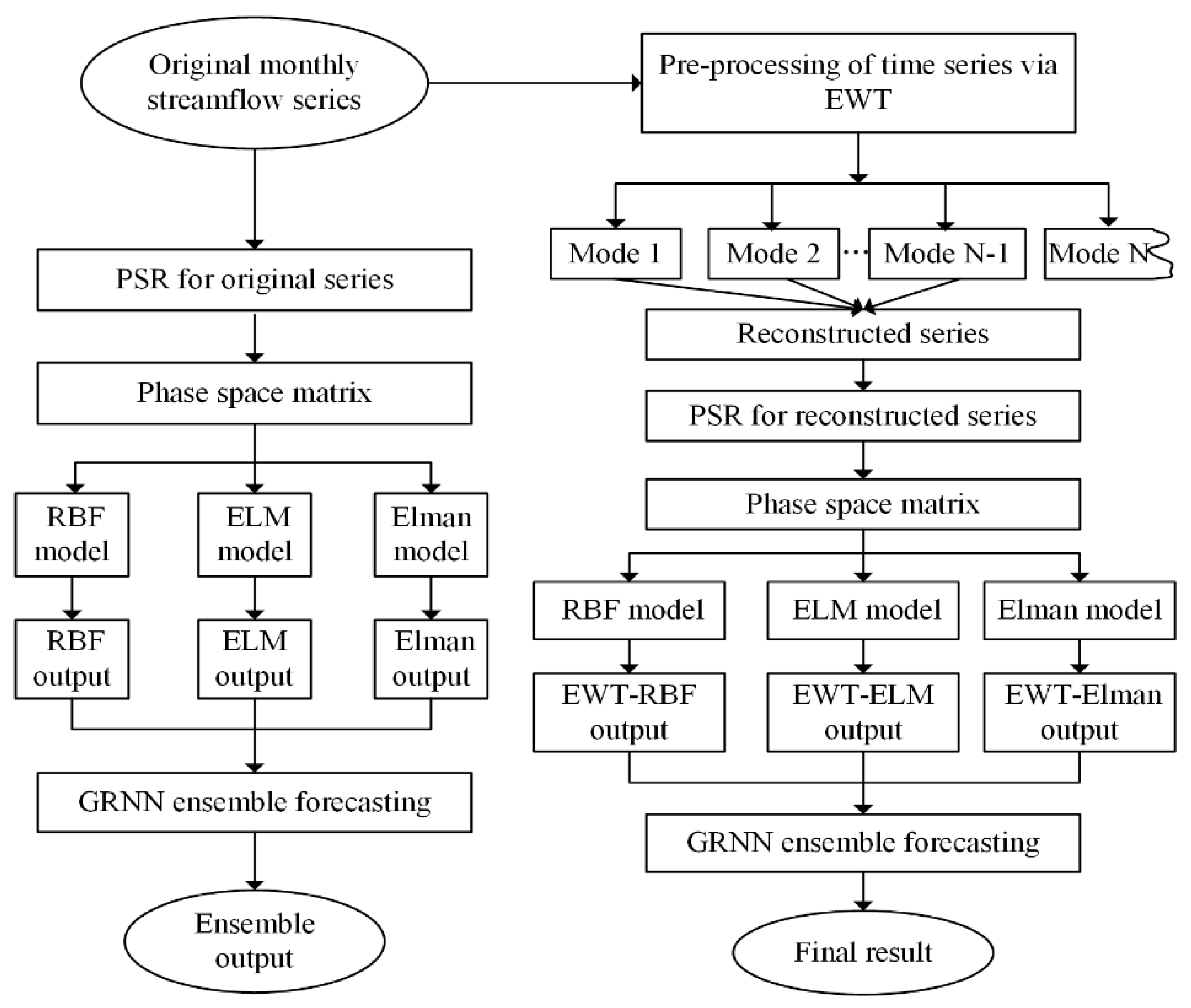
Figure 2 illustrates the detailed procedures of schematic structures of the various models used in this study. The proposed EWT-GNE model could be implemented in four steps. The first step was the denoising process of the original streamflow time series. In this step, the streamflow series was divided into four independent modes using the EWT algorithm. The mode with the highest frequency was removed to eliminate redundant noise. In the second step, the PSR method was used to construct the phase space matrix, namely, the input matrix of the neural networks. In the third step, three individual ANN models, RBF, ELM, and Elman networks, were used to forecast the monthly streamflow time series independently. The three varying architectures of ANNs were chosen because they are three of the most representative ANNs that have been used for forecasting. The RBF network is one of the most widely used FNNs. The ELM network is a new type of SLFNs in which weights and biases are randomly assigned. The Elman network is a type of dynamic recurrent neural network. The last step was to group the results of the three individual models using GRNN. In this part, the forecasted outputs of the RBF, ELM, and Elman networks were taken as input variables of the GNE model. The forecasting result of the GRNN model was the result of the proposed EWT-GNE model. The GRNN network was chosen as an ensemble technique because it has only one parameter to be optimized. Accordingly, errors caused by parameter uncertainty can be decreased. The left portion of Figure 2 illustrates the modelling framework of the models without the EWT denoising technique, while the right portion of Figure 2 illustrates that of the models with the EWT denoising technique.
3. Model Construction and Development
3.1. Study Area and Data Collection
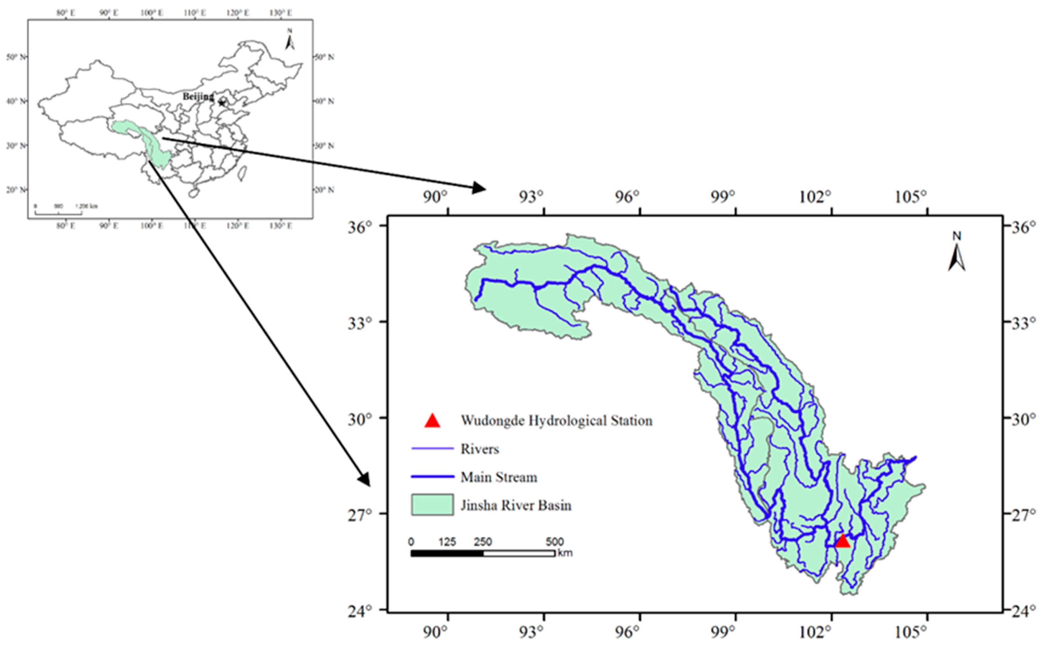
The Jinsha River is located in the upper portion of the Yangtze River and originates in the Tanggula Mountains. It flows through Sichuan, Yunan and Tibet provinces in China. The upper portion of the Yangtze River located in Zhimenda, Yushu in Qinghai Province is called the Jinsha River, the length of which is 2326 km and the height difference is 3280 km. The catchment area of Jinsha River basin is 473,000 km2. The Jinsha River Basin can be subdivided into upper, middle, and lower sections. The monthly streamflow data of the Wudongde hydropower station, which is located in the lower portion of the Jinsha River basin, is studied in this paper. The catchment area of the Wudongde hydropower station is 406,100 km2, which accounts for 86% of the total area of the Jinsha River basin. The average annual discharge is 3810 m3/s and the total runoff is 1200 billion m3. The observed data ranged from January 1958 to December 2012, with a total length of 55 years (660 months). The first 525 months of the streamflow data (January 1958 to September 2001) were selected for training. The remaining 135 months (October 2001 to December 2012) were used for validation. Figure 3 illustrates the locations of the Jinsha River basin and the Wudongde hydrological station.
3.2. Data Preprocessing Using Empirical Wavelet Transform
Before submitting the streamflow series into the forecasting model, the original series was preprocessed using EWT. The original streamflow series was divided into four independent modes. The mode with the highest frequency was discarded. A visual representation of the decomposed subseries and the comparison between the original and denoised series is shown in Figure 4. Following preprocessing, the peaks of the original series were weakened and the troughs were lowered. The oscillations of the monthly streamflow time series were eliminated to a certain extent using EWT.
3.3. Determination of Phase Space Reconstruction Parameters
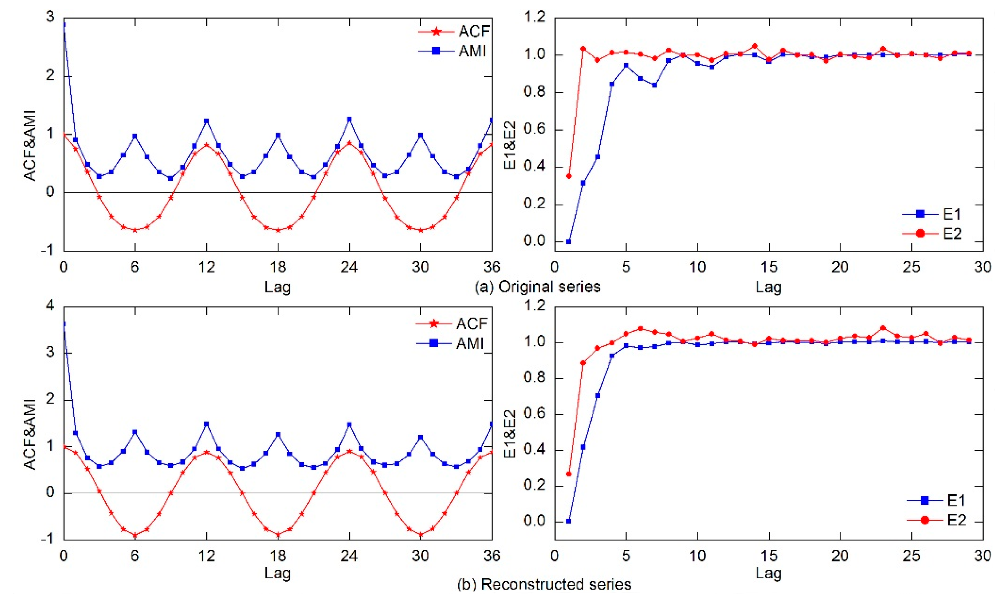
After the denoising process was completed, the one-dimensional denoised streamflow series was reconstructed into a multi-dimensional phase space matrix for forecasting. To determine the delay time of the PSR method, the ACF and AMI values of the original and reconstructed series were calculated. As can be seen in Figure 5, for both the original and the reconstructed series, the AMI values reached the first minimum at lag 3; the ACF values also attained zero. Because the ACF and AMI values gave the same determination of delay time , was chosen as 3 for both the original and the reconstructed time series. After determining the delay time, the Cao method was used to determine the embedded dimension m. As can be seen in Figure 5, because E1(m) almost stopped changing when m was greater than 11, m was chosen as 12 for the original time series, while 8 was chosen for the reconstructed series. After the determination of and m, the maximum Lyapunov exponent was computed for both series. was calculated as 2.263 and 4.142 for the original series and the reconstructed series, respectively. Since the largest Lyapurov exponent was determined to be positive, the streamflow series was identified as chaotic. Additionally, the maximum Lyapunov exponent of the original series was much larger than the reconstructed series, which demonstrated that the reconstructed streamflow time series was less disordered and unsystematic than the original time series, according to chaos theory. Discarding the mode with the highest frequency eliminated the redundant noises of the original monthly streamflow time series. Subsequently, the EWT method could be used as a data preanalysis technique in the forecasting of the monthly streamflow series in this study.
3.4. Parameter Settings of Different ANNs
The diversity of the submodels was realized through the use of various ANN architectures. For the three submodels, the total number of hidden neurons was determined using a gird search (GS) algorithm to assure fair and valid comparisons. The search range was set as , where n denotes the number of input neurons, m is set as if n is bigger than 10; otherwise m was set at 1. The searching step was set at 1. The transfer functions of hidden and output layers were of sigmoid and linear types for the Elman neural networks, respectively, while that of the hidden layer of the ELM network was linear. With regard to the RBF neural network, the spreads ranged from 0.1 to 4.0, with 0.1 increment to obtain the best forecasting performance. The spread was the only parameter to be optimized for the GRNN network. The spreads ranged from 0.02 to 0.1, with 0.01 increment. The optimal parameters for neural networks used in this study for streamflow forecasting are shown in Table 1.
4. Results and Analysis
The comparison and analysis of results can be divided into four steps. First, the comparisons between the methods with and without EWT were conducted to demonstrate the effectiveness of the EWT-based preprocessing method in increasing the accuracy of streamflow time series forecasting. Second, the performance of the three ANN models, e.g., the RBF, Elman, and ELM models, were analyzed to investigate their ability in monthly streamflow forecasting as well as to recommend the most appropriate model. Thirdly, comparisons among the predictions of the various individual and ensemble models were investigated to verify the efficiency of the ensemble techniques. Finally, the performance of the various ensemble techniques, including SAE, WAE, and GNE, were compared to highlight the effectiveness of the GRNN-based ensemble technique.
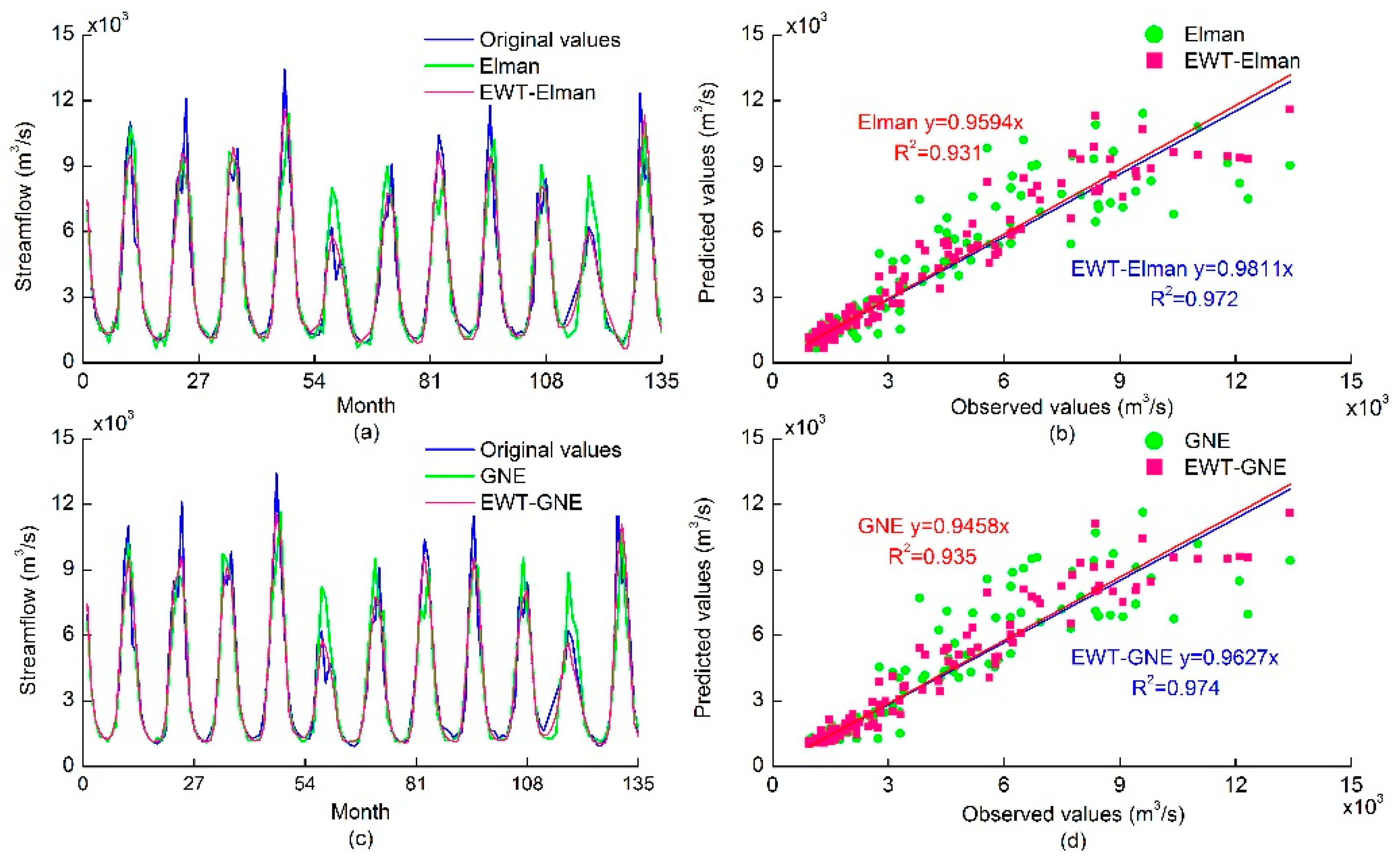
The performance evaluation indices of the 12 models developed in this study, including RBF, ELM, Elman, SAE, WAE, and GNE model, with and without the EWT algorithm, in the training and validation periods are shown in Table 2 and Table 3, respectively. It can be concluded from the preliminary analysis of results between the non-denoising models and the EWT-based models that the performances of the latter were superior to that of the former in terms of the four performance indices. It can be seen from Table 2 and Table 3 that the EWT-based models performed much better than the corresponding non-denoising models. The RMSE, MAE, and MAPE values of the former were all smaller than the latter, while the R value was significantly larger. To display the efficiency of the EWT-based denoising technique, the model performance of the Elman and GNE models with and without EWT in the validation period are shown in Figure 6, where the solid lines on the left represent both the predicted and the observed values, while the right shows the scatter plots. It can be seen from Figure 6 that the EWT-based models (EWT-Elman and EWT-GNE) approximated the original streamflow time series better than the corresponding non-denoising models (Elman and GNE), and the scatters distributed more tightly around the least-square regression line.
To further demonstrate variations in the forecasting performance between the non-denoising models and the EWT-based models, the improved percentages between the two kinds of methods were calculated. The RMSE, MAE, R, and MAPE differences within the EWT-Elman model and the Elman model were 33.22%, 27.77%, 3.39%, 11.89% in the training stage and 36.48%, 31.82%, 3.39%, 27.89% in the validation stage, respectively. For the EWT-GNE model and the GNE models, the RMSE, MAE, R, and MAPE differences were 35.55%, 32.27%, 2.75%, 24.16% and 36.56%, 29.99%, 5.77%, 22.93% in the training and validation stages, respectively. The comparisons between the EWT-based models and the non-denoising models have demonstrated that the EWT denoising process is effective in improving the prediction accuracy of the monthly streamflow.
From the results of Table 2 and Table 3, it can also be seen that the Elman model performed the best in comparison with the RBF and ELM models; additionally, the performance of the RBF model was the worst. The differences between ELM and Elman models were not significant with respect to RMSE, MAE, MAPE, and R criteria. The RMSE, MAE, MAPE, and R of the Elman model consistently performed either equal to or better than the ELM model. The improvements of the RMSE, MAE, MAPE, and R of the Elman model to ELM model were 1.44%, 1.95%, −0.10%, and 7.81% in the validation stage, respectively.
It can also be seen in Table 2 and Table 3 that all ensemble models performed better than the individual models. The ensemble models (GNE and EWT-GNE) performed better than the corresponding best-performing individual model (Elman and EWT-Elman). The RMSE, MAE, R ,and MAPE differences between the GNE and Elman models were 11.23%, 11.20%, 1.31%, 12.24% in the training stage and 3.62%, 5.49%, 0.74%, 12.35% in the validation stage. In contrast, those between the EWT-GNE and EWT-Elman models were 14.33%, 16.73%, 0.68%, 24.46% in the training stage and 3.75%, 2.96%, 0.35%, 6.32% in the validation stage, which demonstrated the effectiveness of the proposed GRNN-ensemble technique in enhancing the predicting ability of ANN models.
From a detailed comparison of the different ensemble models with EWT, according to Table 2 and Table 3, it can be seen that the four indices of both the EWT-WAE and EWT-GNE models were superior to those of the EWT-SAE model. The EWT-GNE model performed slightly better than the EWT-WAE model. The improvement of RMSE, MAE, R, and MAPE was 11.61%, 3.38%, 0.58%, −11.22% in the training stage and 0.73%, −9.52%, 0.03%, −18.68% in the validation stage between EWT-WAE and EWT-GNE models. Additionally, to display the differences between the various ensemble models, the forecasting results of the EWT-SAE, EWT-WAE, and EWT-GNE models are shown in Figure 7. From the illustrations of Figure 7, it can be seen that the predicted values of the EWT-GNE approximated the observed values better than the EWT-SAE model, with the scatters distributed more tightly around the regression line. Thus, the superiority of the proposed GRNN-based ensemble technique over the other ensemble techniques was demonstrated.
5. Conclusions
The present study developed and tested an ANN ensemble model for monthly streamflow forecasting through an application to a case study in China. Three neural network architectures (RBF, ELM, and Elman) were used as sub-ANNs for forecasting. Results demonstrate that all three ANNs performed well, with the best performance achieved by the Elman network. To improve the generalizability and prediction accuracy of the ANNs, various ensemble techniques as the SAE, the WAE, and the GNE were proposed to combine the outputs of the sub-ANNs. The ensemble models achieved better prediction results compared with individual models, with the GRNN-ensemble model having performed the best. As a result of the volatility of the monthly streamflow time series, EWT was used to filter noise. The denoised streamflow time series was less disordered and unsystematic than the original time series according to chaos theory. The models with the EWT-based denoising process outperformed the non-denoising ones. Overall, results show that the proposed EWT-GNE model can be used as a successful tool for monthly streamflow forecasting. The proposed GRNN-ensemble technique can decrease the unpredictability of single ANN forecasting models, and the EWT algorithm can filter the noises of the streamflow series, providing more accurate forecasting results.
In the future, one can apply the techniques developed in this study to streamflow data in different time scales and from other hydrological stations. Hydro-meteorological data such as rainfall [8,14], precipitation, and streamflow data from adjacent hydrological stations [30] can be considered as model inputs to enhance streamflow forecasting accuracy. Additionally, the newest machine learning techniques, such as deep learning [36], can be considered in terms of streamflow forecasting.
Author Contributions
J.Z. and T.P. designed the experiments; T.P. wrote the draft of the paper; C.Z. prepared the figures; J.Z. and N.S. provided useful advices and made some corrections. All authors read and approved the final manuscript.
Funding
This work is supported by the Key Program of the Major Research Plan of the National Natural Science Foundation of China (No. 91547208), the National Natural Science Foundation of China (No. 51579107), and the National Key R&D Program of China (2016YFC0402708, 2016YFC0401005).
Conflicts of Interest
The authors declare no conflict of interest.
References
- Hong, M.; Wang, D.; Wang, Y.; Zeng, X.; Ge, S.; Yan, H.; Singh, V.P. Mid- and long-term runoff predictions by an improved phase-space reconstruction model. Environ. Res. 2016, 148, 560–573. [Google Scholar] [CrossRef] [PubMed]
- Peng, T.; Zhou, J.; Zhang, C.; Fu, W. Streamflow forecasting using empirical wavelet transform and artificial neural networks. Water 2017, 9, 406. [Google Scholar] [CrossRef]
- Hong, W.C.; Pai, P.F. Potential assessment of the support vector regression technique in rainfall forecasting. Water Resour. Manag. 2007, 21, 495–513. [Google Scholar] [CrossRef]
- Solomatine, D.P.; Ostfeld, A. Data-driven modelling: Some past experiences and new approaches. J. Hydroinform. 2008, 10, 3–22. [Google Scholar] [CrossRef]
- Pumo, D.; Viola, F.; Noto, L.V. Generation of natural runoff monthly series at ungauged sites using a regional regressive model. Water 2016, 8, 209. [Google Scholar] [CrossRef] [Green Version]
- Pumo, D.; Conti, F.L.; Viola, F.; Noto, L.V. An automatic tool for reconstructing monthly time-series of hydro-climatic variables at ungauged basins. Environ. Model. Softw. 2017, 95, 381–400. [Google Scholar] [CrossRef]
- Zhang, C.; Zhou, J.; Li, C.; Fu, W.; Peng, T. A compound structure of ELM based on feature selection and parameter optimization using hybrid backtracking search algorithm for wind speed forecasting. Energy Convers. Manag. 2017, 143, 360–376. [Google Scholar] [CrossRef]
- Chen, L.; Singh, V.P.; Guo, S.; Zhou, J.; Ye, L. Copula entropy coupled with artificial neural network for rainfall–runoff simulation. Stoch. Environ. Res. Risk Assess. 2014, 28, 1755–1767. [Google Scholar] [CrossRef]
- Chang, F.J.; Chen, P.A.; Lu, Y.R.; Huang, E.; Chang, K.Y. Real-time multi-step-ahead water level forecasting by recurrent neural networks for urban flood control. J. Hydrol. 2014, 517, 836–846. [Google Scholar] [CrossRef]
- Hosseini-Moghari, S.M.; Araghinejad, S. Monthly and seasonal drought forecasting using statistical neural networks. Environ. Earth Sci. 2015, 74, 397–412. [Google Scholar] [CrossRef]
- Zhou, T.; Wang, F.; Yang, Z. Comparative analysis of ANN and SVM models combined with wavelet preprocess for groundwater depth prediction. Water 2017, 9, 781. [Google Scholar] [CrossRef]
- Yu, Y.; Zhang, H.; Singh, V. Forward prediction of runoff data in data-scarce basins with an improved ensemble empirical mode decomposition (EEMD) model. Water 2018, 10, 388. [Google Scholar] [CrossRef]
- Wang, W.C.; Chau, K.W.; Qiu, L.; Chen, Y.B. Improving forecasting accuracy of medium and long-term runoff using artificial neural network based on EEMD decomposition. Environ. Res. 2015, 139, 46–54. [Google Scholar] [CrossRef] [PubMed]
- Zhu, S.; Zhou, J.; Ye, L.; Meng, C. Streamflow estimation by support vector machine coupled with different methods of time series decomposition in the upper reaches of Yangtze river, China. Environ. Earth Sci. 2016, 75, 531. [Google Scholar] [CrossRef]
- Seo, Y.; Kim, S.; Kisi, O.; Singh, V.P. Daily water level forecasting using wavelet decomposition and artificial intelligence techniques. J. Hydrol. 2015, 520, 224–243. [Google Scholar] [CrossRef]
- Gilles, J. Empirical wavelet transform. IEEE Trans. Signal Process. 2013, 61, 3999–4010. [Google Scholar] [CrossRef]
- Hu, J.; Wang, J. Short-term wind speed prediction using empirical wavelet transform and Gaussian process regression. Energy 2015, 93, 1456–1466. [Google Scholar] [CrossRef]
- Wang, J.; Hu, J. A robust combination approach for short-term wind speed forecasting and analysis—Combination of the ARIMA (Autoregressive Integrated Moving Average), ELM (Extreme Learning Machine), SVM (Support Vector Machine) and LSSVM (Least Square SVM) forecasts using a GPR (Gaussian Process Regression) model. Energy 2015, 93, 41–56. [Google Scholar]
- Zhao, X.; Chen, X.; Xu, Y.; Xi, D.; Zhang, Y.; Zheng, X. An EMD-based chaotic least squares support vector machine hybrid model for annual runoff forecasting. Water 2017, 9, 153. [Google Scholar] [CrossRef]
- Guo, J.; Zhou, J.; Qin, H.; Zou, Q.; Li, Q. Monthly streamflow forecasting based on improved support vector machine model. Expert Syst. Appl. 2011, 38, 13073–13081. [Google Scholar] [CrossRef]
- Hu, Z.; Zhang, C.; Luo, G.; Teng, Z.; Jia, C. Characterizing cross-scale chaotic behaviors of the runoff time series in an inland river of Central Asia. Quat. Int. 2013, 311, 132–139. [Google Scholar] [CrossRef]
- Ouyang, Q.; Lu, W.; Xin, X.; Zhang, Y.; Cheng, W.; Yu, T. Monthly rainfall forecasting using EEMD-SVR based on phase-space reconstruction. Water Resour. Manag. 2016, 30, 2311–2325. [Google Scholar] [CrossRef]
- Pumo, D.; Francipane, A.; Conti, F.L.; Arnone, E.; Bitonto, P.; Viola, F.; La Loggia, G.; Noto, L.V. The SESAMO early warning system for rainfall-triggered landslides. J. Hydroinform. 2016, 18, 256–276. [Google Scholar] [CrossRef] [Green Version]
- Ren, Y.; Suganthan, P.N.; Srikanth, N. Ensemble methods for wind and solar power forecasting—A state-of-the-art review. Renew. Sustain. Energy Rev. 2015, 50, 82–91. [Google Scholar] [CrossRef]
- Jovanović, R.Ž.; Sretenović, A.A.; Živković, B.D. Ensemble of various neural networks for prediction of heating energy consumption. Energy Build. 2015, 94, 189–199. [Google Scholar] [CrossRef]
- Lin, G.F.; Chen, L.H. A non-linear rainfall-runoff model using radial basis function network. J. Hydrol. 2004, 289, 1–8. [Google Scholar] [CrossRef]
- Huang, G.B.; Zhu, Q.Y.; Siew, C.K. Extreme learning machine: A new learning scheme of feedforward neural networks. In Proceedings of the IEEE International Joint Conference on Neural Networks, Budapest, Hungary, 25–29 July 2004; Volume 982, pp. 985–990. [Google Scholar]
- Elman, J.L. Finding structure in time. Cogn. Sci. 1990, 14, 179–211. [Google Scholar] [CrossRef]
- Specht, D.F. A general regression neural network. IEEE Trans. Neural Netw. 1991, 2, 568–576. [Google Scholar] [CrossRef] [PubMed]
- Chen, L.; Ye, L.; Singh, V.; Asce, F.; Zhou, J.; Guo, S. Determination of input for artificial neural networks for flood forecasting using the copula entropy method. J. Hydrol. Eng. 2014, 19, 217–226. [Google Scholar] [CrossRef]
- Packard, N.H.; Crutchfield, J.P.; Farmer, J.D.; Shaw, R.S. Geometry from a time series. Phys. Rev. Lett. 1980, 45, 712. [Google Scholar] [CrossRef]
- Cao, L. Practical method for determining the minimum embedding dimension of a scalar time series. Phys. D Nonlinear Phenom. 1997, 110, 43–50. [Google Scholar] [CrossRef]
- Wu, C.L.; Chau, K.W.; Fan, C. Prediction of rainfall time series using modular artificial neural networks coupled with data-preprocessing techniques. J. Hydrol. 2010, 389, 146–167. [Google Scholar] [CrossRef]
- Rosenstein, M.T.; Collins, J.J.; Luca, C.J.D. A practical method for calculating largest Lyapunov exponents from small data sets. Phys. D Nonlinear Phenom. 1993, 65, 117–134. [Google Scholar] [CrossRef]
- Peng, T.; Zhou, J.; Zhang, C.; Zheng, Y. Multi-step ahead wind speed forecasting using a hybrid model based on two-stage decomposition technique and AdaBoost-extreme learning machine. Energy Convers. Manag. 2017, 153, 589–602. [Google Scholar] [CrossRef]
- Bai, Y.; Chen, Z.; Xie, J.; Li, C. Daily reservoir inflow forecasting using multiscale deep feature learning with hybrid models. J. Hydrol. 2016, 532, 193–206. [Google Scholar] [CrossRef]
Figure 1.
The structure of the GNE model based on RRF, ELM and Elman networks.

Figure 2.
A schematic view of the modeling framework.

Figure 3.
Locations of the Jinsha River basin and the Wudongde hydrological station.

Figure 4.
Visual representation of the decomposed subseries and the comparison between the original and reconstructed series.
Figure 4.
Visual representation of the decomposed subseries and the comparison between the original and reconstructed series.

Figure 5.
The auto-correction function (ACF) & Average Mutual Information (AMI) values and Cao method results plot for the original and reconstructed streamflow series.
Figure 5.
The auto-correction function (ACF) & Average Mutual Information (AMI) values and Cao method results plot for the original and reconstructed streamflow series.

Figure 6.
Forecasting results of the Elman (GNE) and EWT-Elman (EWT-GNE) models in the validation stage.
Figure 6.
Forecasting results of the Elman (GNE) and EWT-Elman (EWT-GNE) models in the validation stage.

Figure 7.
Forecasting results of the simple averaging ensemble (SAE), weighted averaging ensemble (WAE) and GRNN-based ensemble (GNE) models with EWT in the validation stage.
Figure 7.
Forecasting results of the simple averaging ensemble (SAE), weighted averaging ensemble (WAE) and GRNN-based ensemble (GNE) models with EWT in the validation stage.


Table 1.
Optimal parameters of the ANN models used for streamflow forecasting.
| Models | RBF | EWT-RBF | ELM | EWT-ELM | Elman | EWT-Elman | GNE | EWT-GNE |
|---|---|---|---|---|---|---|---|---|
| Neurons | 20 | 20 | 43 | 35 | 9 | 20 | -- | -- |
| Spread | 1.4 | 1.8 | -- | -- | -- | -- | 0.045 | 0.029 |
Table 2.
The forecasting results of the models in the training period.
| Models | RMSE (m3/s) | MAE (m3/s) | R | MAPE (%) | Models | RMSE (m3/s) | MAE (m3/s) | R | MAPE (%) |
|---|---|---|---|---|---|---|---|---|---|
| RBF | 1175.70 | 710.11 | 0.931 | 17.751 | EWT-RBF | 748.72 | 480.94 | 0.973 | 13.508 |
| ELM | 1138.34 | 711.62 | 0.935 | 19.445 | EWT-ELM | 712.07 | 462.07 | 0.975 | 13.046 |
| Elman | 1071.81 | 641.72 | 0.943 | 15.380 | EWT-Elman | 715.71 | 463.51 | 0.975 | 13.551 |
| SAE | 1103.51 | 648.95 | 0.939 | 15.513 | EWT-SAE | 711.13 | 443.49 | 0.975 | 11.362 |
| WAE | 1070.36 | 574.04 | 0.943 | 12.268 | EWT-WAE | 693.70 | 399.46 | 0.976 | 9.204 |
| GNE | 920.53 | 548.81 | 0.958 | 13.055 | EWT-GNE | 613.16 | 385.95 | 0.982 | 10.237 |
Table 3.
The forecasting results of the models in the validation period.
| Models | RMSE (m3/s) | MAE (m3/s) | R | MAPE (%) | Models | RMSE (m3/s) | MAE (m3/s) | R | MAPE (%) |
|---|---|---|---|---|---|---|---|---|---|
| RBF | 1351.04 | 796.64 | 0.898 | 20.342 | EWT-RBF | 854.68 | 574.94 | 0.959 | 17.446 |
| ELM | 1308.82 | 796.89 | 0.903 | 19.350 | EWT-ELM | 833.07 | 554.03 | 0.961 | 15.679 |
| Elman | 1292.60 | 796.78 | 0.906 | 20.045 | EWT-Elman | 821.11 | 543.21 | 0.962 | 14.455 |
| SAE | 1293.75 | 752.28 | 0.906 | 17.159 | EWT-SAE | 820.40 | 538.90 | 0.962 | 13.699 |
| WAE | 1264.56 | 677.82 | 0.910 | 14.016 | EWT-WAE | 796.13 | 481.35 | 0.965 | 11.410 |
| GNE | 1246.47 | 753.16 | 0.913 | 17.602 | EWT-GNE | 790.35 | 527.15 | 0.965 | 13.541 |
© 2018 by the authors. Licensee MDPI, Basel, Switzerland. This article is an open access article distributed under the terms and conditions of the Creative Commons Attribution (CC BY) license (http://creativecommons.org/licenses/by/4.0/).
Share and Cite
MDPI and ACS Style
Zhou, J.; Peng, T.; Zhang, C.; Sun, N. Data Pre-Analysis and Ensemble of Various Artificial Neural Networks for Monthly Streamflow Forecasting. Water 2018, 10, 628. https://doi.org/10.3390/w10050628
AMA Style
Zhou J, Peng T, Zhang C, Sun N. Data Pre-Analysis and Ensemble of Various Artificial Neural Networks for Monthly Streamflow Forecasting. Water. 2018; 10(5):628. https://doi.org/10.3390/w10050628
Chicago/Turabian StyleZhou, Jianzhong, Tian Peng, Chu Zhang, and Na Sun. 2018. "Data Pre-Analysis and Ensemble of Various Artificial Neural Networks for Monthly Streamflow Forecasting" Water 10, no. 5: 628. https://doi.org/10.3390/w10050628
Note that from the first issue of 2016, this journal uses article numbers instead of page numbers. See further details here.