Article

Integrated Effects of Land Use and Topography on Streamflow Response to Precipitation in an Agriculture-Forest Dominated Northern Watershed

1
North China University of Water Resources and Electric Power, Zhengzhou 450045, China
2
State Key Laboratory of Hydroscience and Engineering, Tsinghua University, Beijing 100084, China
3
Henan Key Laboratory of Water Environment Simulation and Treatment, Zhengzhou 450046, China
4
EcoLab, Université de Toulouse, CNRS, INPT, UPS, Toulouse, France, Avenue de l’Agrobiopole, 31326 Castanet Tolosan Cedex, France
5
Research Faculty of Agriculture, Hokkaido University, Sapporo 0608589, Japan
*
Authors to whom correspondence should be addressed.
Water 2018, 10(5), 633; https://doi.org/10.3390/w10050633
Submission received: 2 April 2018 / Revised: 2 May 2018 / Accepted: 7 May 2018 / Published: 13 May 2018
(This article belongs to the Section Hydrology)

Abstract

:
Based on statistical analysis, baseflow separation and wavelet analysis, this research was carried out in Shibetsu River Watershed (SRW), Eastern Hokkaido, Japan, to investigate the integrated effects of land use and topography on streamflow response to precipitation. The agriculture-dominated sub-watershed (AW) showed coupled flat topography/agriculture characteristics, the forest-dominated sub-watershed (FW) had coupled steep topography/forest characteristics, and the mixed agriculture-forested sub-watershed (AFW) had mixed flat topography/agriculture and steep topography/forest characteristics. Precipitation variability is characterized by 6-months and 1-year periods. Coupled forest land/steep topography of the FW can increase surface runoff due to forest surface soil water repellency and steep slope, and might receive more external water and higher precipitation that resulted in the highest baseflow and total streamflow compared with other sub-watersheds. Coupled forest land/steep topography can cause higher monthly streamflow variability than coupled agricultural land/flat topography. The FW streamflow is characterized by 3–4 months, 6 months, and 1-year periods. The AW streamflow is only characterized by 3–4 months and 6 months periods. Coupled agricultural land/flat topography produced similar magnitude of baseflow during snowmelt season (March–May) and rainfall season (July–September), which resulted in the losing of annual periodicity in AW streamflow. The coupled forest land/steep topography can increase synchronicity in precipitation and streamflow at annual and monthly scales than coupled agricultural land/flat topography, except in 2007 under wet antecedent conditions when pasture land has lower rainfall interception and lower surface soil infiltration capacity. The coupled forest land/steep topography can increase time lags between precipitation and streamflow compared to coupled agricultural land/flat topography.

1. Introduction

A scientific understanding of streamflow generation is important for effective water management, e.g., flood control, drought relief, water quality protection, aquatic ecosystem reservation, and public water security [1,2]. Streamflow generation is a result of many influencing factors, e.g., land use, topography, soils, and climate (i.e., precipitation and temperature) [3,4,5]. The need for a better understanding of the effect of these factors on streamflow response to precipitation has been recognized for decades. For watersheds under similar climate and soils conditions, topography and land use could be the dominant factors controlling streamflow response to precipitation.
The effect of land use type on streamflow generation has been widely reported around the world [6]. Land use types have significant impact on hydrological processes, such as evapotranspiration, surface runoff, and consequently, streamflow generation [7]. Land use may significantly influence the temporal variations of streamflow in a watershed [8,9]. For example, forest may produce higher or lower stream water yield than pasture or other agricultural lands because forest region has higher precipitation interception, evaporation, transpiration and higher soil infiltration [10]. Previous studies found that pasture or agricultural lands could have higher streamflow yields and amplitude, while forest generally have lower water yield compared with pasture [11,12,13,14]. However, it was also reported that pasture can reduce streamflow in dry periods because it has low infiltration rate caused by grazing or agricultural machinery [15]. In pasture land, the decreases in soil water and groundwater recharge could offset the low evapotranspiration. Bruijnzeel [15] reported that conversion of forest to agriculture decreased baseflow, while Ma et al. [16] reported afforestation could increase baseflow. The impact of land use on streamflow generation might vary from region to region, especially when it is coupled with other factors in a watershed.
Topography is another important factor influencing streamflow generation. For example, topography can determine when surface flow and subsurface flow enter into stream. Steep topography could result in quick response [17]. With the increase of mean slope in the watershed, subsurface flow and quick flow proportions could increase, whereas surface flow proportion could decrease [3]. Tetzlaff et al. [18] reported that topography could significantly affect baseflow processes and transmission rates of water, especially in areas of high relief ratio. In addition, topography could influence soil and bedrock development, thus, influence the subsurface flow storage [1]. The influences of land use on streamflow yields and dynamics could be mitigated or amplified by watershed topographic variations [1].
Most commonly, impacts of land use or topography on streamflow generation were examined separately from paired-watersheds with different land use and similar topography or different topography but similar land use [8,19]. However, watersheds might be characterized by contrasting land use and topography, e.g., agriculture is usually developed in flat regions, while forest exists in steep regions. Usually, forest located in steep regions are critical zones for soil erosion and could be protected by governmental laws, whereas forest in flat region could be converted to agriculture around the world [20,21,22]. For example, forest in flat regions was converted to pasture and agriculture in central Veracruz, Mexico [23]. However, the coupled flat topography/agriculture and the coupled steep topography/forest effects on streamflow generation are still not fully understood and deserve further studies.
The agriculture-forest dominated Shibetsu River Watershed (SRW, Eastern Hokkaido, Japan) has coupled flat topography/agriculture and coupled steep topography/forest characteristics. In this study, six years’ records of daily precipitation and streamflow data (2003–2008) were collected for three sub-watersheds within SRW with similar soil properties, but different land use/topography combinations: the agricultural sub-watershed (AW) showed coupled flat topography/agriculture characteristics, the forestry sub-watershed (FW) had coupled steep topography/forest characteristics, and the mixed agriculture and forest dominated sub-watershed (AFW) developed agriculture in flat regions, while preserved the forest in the steep region. By comparing precipitation and streamflow data of the three neighboring sub-watersheds in Shibetsu River Watershed, main objectives of this study are to understand the coupled effect of land use and topography on streamflow variability and streamflow response to precipitation.
In the following sections, we first give a detailed description of the study sites, data collection, and data analysis methods including snowmelt calculation, baseflow separation, statistical analysis, and wavelet analysis in Section 2. Then, results for the precipitation and streamflow variability characteristics and theirs relationships are presented in Section 3, and the integrated effects of land use and topography on streamflow variability and streamflow response to precipitation are discussed in Section 4. Finally, conclusions are given in Section 5.

2. Material and Methods

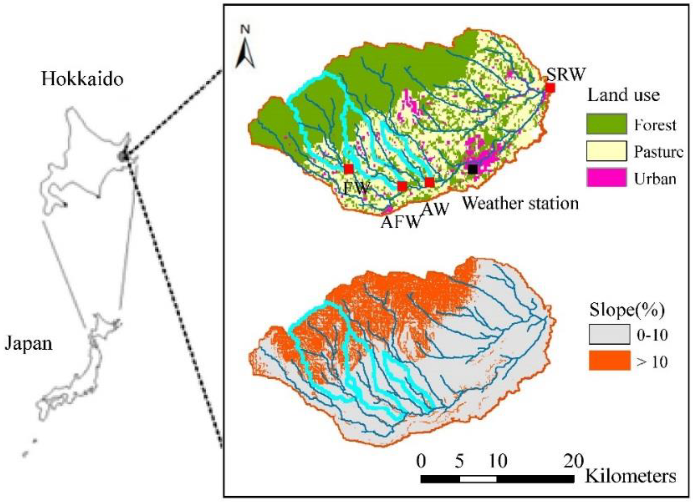
2.1. Study Site and Data Collection

This study was carried out in the Shibetsu River Watershed (SRW, 672 km2, eastern Hokkaido, Japan) (Figure 1). Annual mean precipitation is around 1130 mm·year−1 and temperature is about 5.0 °C (Japan Meteorological Agency, http://www.jma.go.jp). In the study site, winter is cold and the snow period is long (December–April). The external groundwater (EXT) from neighboring watersheds entered into the SRW as reported by Jiang et al. [24]. As a result, annual streamflow amount is usually higher than annual precipitation. The soils in SRW are formed from volcanic ashes, the major soil types of the SRW include 3.3% Peat soils (6.6% clay and 61% sand), 14% Regosolic Kuroboku soils (33% clay and 64% sand), 21% Brown Forest soils (19% clay, 54.63% sand and 10% gravel), 46% Kuroboku soils (5.0% clay and 65% sand), 9.1% Brown Lowland soils (3.3% clay and 65% sand), 4.5% Regosols (2.4% clay and 85% sand) and 2.6% Grey Lowland soils (5.5% clay and 52% sand). Their detailed properties can be found in Jiang et al. [24]. The land uses of SRW were published by Japanese Geographical Survey Institute (JGSI, http://nlftp.mlit.go.jp/ksj/jpgis/jpgis_datalist.html) and are shown in Figure 1 and Table 1. The forest (Larix kaempfer L., 53.7%) and agricultural pasture (Phleum pratense L., 40.8%) are the main land uses in SRW. The slopes of SRW are calculated from 50 m mesh digital elevation model (DEM) published by JGSI. About 30% of SRW is steep with slopes greater than 10%, as shown in Figure 1b. Main land use in the flat terrain (with slope less than 10%) is agriculture and accounts for the other 70% of the watershed (Figure 1, Table 1). The elevation of the SRW ranges from 4 m to 1059 m. The relief ratio (defined as difference between maximum and minimum elevation divided by its maximum stream length in a watershed) is 0.017 in SRW.
Three sub-watersheds located in the SRW were selected for this study (Figure 1 and Table 1). The three sub-watersheds had coupled land use and topography characteristics and were adjacent to reduce the spatial heterogeneity of soils. The agriculture-dominated sub-watershed (AW) covers 14.3 km2 and is dominated by agricultural pasture (73.5%). The forest-dominated sub-watershed (FW) covers 70.0 km2, and a large proportion (84.4%) is covered by forest. The mixed agriculture-forest sub-watershed (AFW) covers 36.6 km2 and consists of mixed agriculture (58.9%) and forest (37.1%). For the AW, the relief ratio is 0.015, and the flat topography (slope less than 10%) contributed about 97.5% of the total area. The FW had a relief value of 0.055, and steep topography (slope higher than 10%) covers 62.8% of the total area. The relief ratio of AFW is 0.036. About 79.7% of the AFW was flat while the other region was steep. As illustrated in Figure 1 and Table 1, AW showed coupled flat topography/agriculture characteristics, the FW had coupled steep topography/forest characteristics, and the AFW was similar with SRW, i.e., developing agriculture in flat regions, while preserving the forest in the steep region. The soils and belowground rocks were formed from volcanic ash in SRW (http://iggis1.muse.aist.go.jp/en/top.htm). Most soils in SRW are characterized with high sand content (>50%) and low clay content (<20%) [25]. Thus, soil is not considered as a key factor to streamflow generation in this study. The presence of EXT and volcanic substrata indicate that the underground water network is complicated. Correspondingly, hydrological modeling is quite challenging in SRW.
Daily meteorological and streamflow data in six years from 2003 to 2008 were collected for the three sub-watersheds and the whole watershed. Daily meteorological data (precipitation, temperature, and the maximum depth of accumulated snow) in Nakashibetsu Station (Figure 1) were obtained from Japan Meteorological Agency (http://www.jma.go.jp/jma/). The Nakashibetsu weather station was selected because data of maximum depth of accumulated snow were available in this weather station. The time when maximum depth of accumulated snow decreased to zero indicated the end of snowmelt. The streamflow rates at the three sub-watersheds and the whole watershed outlets were calculated using the relationships between streamflow and water level measured with water sensors (MC-1100W, STS, Sirnach, Switzerland) as recommended by Tachibana and Nasu [26].

2.2. Data Analysis

2.2.1. Snowmelt Calculation

In Hokkaido, Japan, the ground was covered by snow from December to April. However, the timing and rate of snowmelt was not available. Therefore, in this study, the degree-day snowmelt model was used to calculate snowmelt [27]. The critical temperatures for snow/rain separation (T0, °C) is 0 °C in Hokkaido, Japan, as recommended by previous study [27]. Snow accumulated when temperatures <0 °C and snowmelt happened when temperatures >0 °C. In this study, precipitation was considered as rainfall plus snowmelt. The degree-day snowmelt model using a melt factor is used to calculate daily snowmelt amount as:
Ms = D(TT0) and 0 < Ms ≤ Sa, if T > 0 and Sa > 0
Ms = 0, if T ≤ 0 and/or Sa (or R) ≤ 0
where Ms is the snowmelt amount (mm/day); D is melt factor (mm/°C/day); T is air temperature (°C); TT0 is the effective temperature for snowmelt (°C); Sa is the accumulated snow (mm); R is the rainfall (mm).
In this study, a melt factor value of 6 mm/°C/day was calculated based on the end time of snowmelt and used in this study. This is in accordance with the study of Motoyama [27] which reported that melt factor ranged between 5.5–7 mm/°C/day in Hokkaido, Japan. Other factors, such as the fluctuations of temperature and precipitation within a day, solar radiation, and depth of snow cover, might also have strong influences on snowfall and snowmelt amounts [27,28]. However, due to lack of those energy-balance data and direct observations for snowmelt in the study site, the degree-day melt model is used to provide an estimate of snowmelt water amounts at daily time step.

2.2.2. Direct Runoff and Baseflow Separation

The digital filter-based program proposed by Arnold and Allen [29] is adopted in this study to separate direct runoff and baseflow from streamflow. In this digital filter-based program, long waves were considered as baseflow that usually originate from groundwater discharge, while the high frequency streamflow waves were considered as direct runoff. The filter equation can be expressed as:
Q s f , i = λ Q s f , i 1 + 1 + λ 2 ( Q s , i Q s , i 1 )
where Q s f is the direct runoff, i is the day number, Q s is the streamflow, and λ is the filter parameter. In this study, a filter parameter value of 0.925 recommended by Nathan and McMahon [30] was adopted. The baseflow ( Q b ) can then be calculated as:
Q b , i = Q s , i Q s f , i

2.2.3. Precipitation and Streamflow Variability Analysis

Annual and monthly precipitation and streamflow variability were analyzed at the four watersheds according to Carey et al. [31]. On an annual basis, coefficient of variation (Cv) of annual streamflow (QA) and annual precipitation (PA), the ratio of their Cv, CvQA/CvPA, and their correlation coefficients, cor(QA, PA) were calculated. The statistics of CvQA/CvPA and cor(QA, PA) were used to measure annual consistency between streamflow and precipitation.
Statistics of monthly precipitation and streamflow can be used to assess their seasonality and synchronicity. The Cv of monthly precipitation (CvPmo) indicates the difference between dry and wet seasons, whereas the Cv of monthly streamflow (CvQmo) indicates the seasonal streamflow variability. To evaluate the relationship between precipitation and streamflow variation, the ratio of CvQmo/CvPmo and correlation coefficients of cor(Qmo, Pmo) were calculated.
The closer Cv of streamflow to Cv of precipitation, the higher synchronicity of hydrological regimes. The closer the cor(Q, P) to 1, the higher synchronicity of hydrological regimes.

2.2.4. Wavelet Analysis of Daily Precipitation and Streamflow

Wavelet analysis is a widely used method for analyzing features of time series using wavelet transform (WT). Main feature of the WT is that it can localize processes related to time-scale. The continuous wavelet transform (CWT) can particularly achieve the aim of extracting features. Various CWTs were presented in previous literature [32], the CWT adopted in this study is the Morlet transform. The detailed mathematical basis of CWT can refer to Meyer [33] and Torrence and Compo [34]. Wavelet analysis can also be used to check two processes together to find out their relationships. Specifically, the Cross Wavelet Transform (XWT) can be used to check whether regions in time-scale space with high common spectral power have a consistent phase relationship. In this study, XWT is used to estimate the phase difference between the precipitation and stream series. Details about estimating phase difference from XWT can be seen in Torrence and Webster [35] as well as in Torrence and Compo [34]. The Wavelet Coherence (WTC) is another commonly used method to examine two time series together. The WTC is calculated as the square of the cross-spectrum normalized by the individual spectral power. Thus, it can measure the cross-correlation between two time series and give a quantity ranging from 0 to 1. Even when the XWT power of the two series is low, high levels of significance can still be found using WTC. The WTC is considered as an accurate representation of the normalized covariance between the two time series [35]. The Global Wavelet Spectrum (GWS) is defined as the absolute value squared of the WT, which can estimate the variance of the time series at each scale/period and at each time.
In this paper, wavelet analysis is used to characterize and clarify the temporal variability of daily precipitation, streamflow and the relationship between them. In order to apply the CWT, XWT and WTC accurately, the probability distribution should be close to normal distribution [36]. Therefore, the logarithmic transformations were adopted for precipitation and streamflow because they have a log-normal distribution. The Matlab software package named WTC-R15 were used to conduct wavelet analysis, which is accessible at http://noc.ac.uk/marine-data-products/cross-wavelet-wavelet-coherence-toolbox-matlab [36].

3. Results

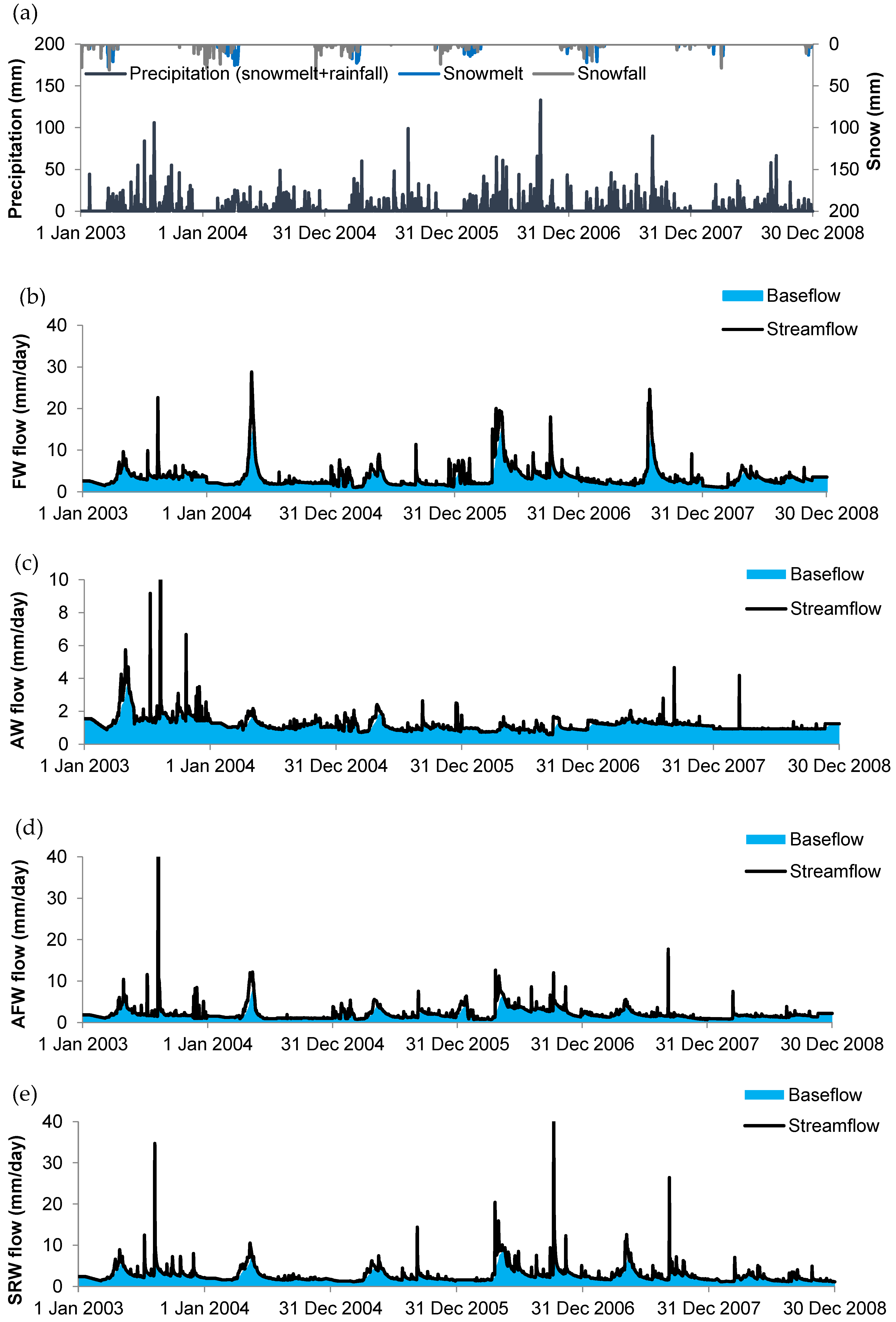
3.1. Temporal Variation of Daily Precipitation

Figure 2a depicts the temporal variation of daily precipitation (including snowmelt and rainfall). Average annual precipitation records in the Shibetsu River Watershed from 2003–2008 were 1050 mm, with the daily maximum value of 133 mm in 10 August 2006. Average annual snowmelt was 150 mm, which contributed about 14% to the annual precipitation. Snowmelt usually starts in late February or early March, and end in middle April. Rainfall also happens during the snowmelt period. Rainfall plus snowmelt during the snowmelt period was about 210 mm, which contributed about 20% to the annual precipitation. The main rainfall season is from July to September, rainfall during this period was about 410 mm, which contributed about 40% to the annual precipitation.

3.2. Precipitation and Streamflow Characteristics

3.2.1. Annual and Monthly Precipitation and Streamflow Characteristics

The area-normalized daily streamflow (expressed in mm) and baseflow of the four watersheds from 2003 to 2008 are shown in Figure 2b–e). Contributions of baseflow and surface flow to the total streamflow are shown in Table 2. Streamflow begins to rise consistently following the snowmelt till discharge peak in late April or early May. During rainy season from June to December, streamflow could rise and recede steeply. The snow season begins in late November, and the surface runoff to streamflow ceases, the streamflow becomes stable and flat during the winter and spring seasons for a long period. The mean daily streamflow is 3.53, 1.24, 2.20, and 2.80 mm, with surface runoff contributions of 0.56, 0.11, 0.38, and 0.38 mm and subsurface flow contributions of 2.97 (84.1%), 1.13 (91.1%), 1.82 (82.7%), and 2.42 (86.4%) mm, respectively, for FW, AW, AFW, and SRW. The large fraction of the subsurface flow was due to that external water from the neighboring watershed entered into the study watershed as groundwater [37].
Statistics of precipitation and streamflow are shown in Table 3, and wide variability of streamflow exists among all watersheds. For the annual and monthly precipitation variability in SRW, the CvPA is 0.22 and CvPmo is 0.83. AW and FW had the similar CvQA and CvQA/CvPA values, which are 0.28 and 1.27 for AW and 0.26 and 1.18 for FW, respectively. However, cor(QA, PA) value is much lower in AW (0.09) compared with FW (0.75). Besides, AFW and SRW had higher cor(QA, PA) values of 0.93 and 0.94 than AW and FW, respectively. For monthly streamflow variability, CvQmo is lowest in AW (0.34) and highest in FW (0.65), AFW and SRW had similar values of 0.59 and 0.54, respectively. Accordingly, the CvQmo/CvPmo is the lowest in AW (0.41) and highest in FW (0.78). The cor(Qmo, Pmo) is the lowest in AW (0.01), FW had a little higher values of 0.06, while AFW and SRW are both higher than FW and AW with the values of 0.10 and 0.21, respectively.

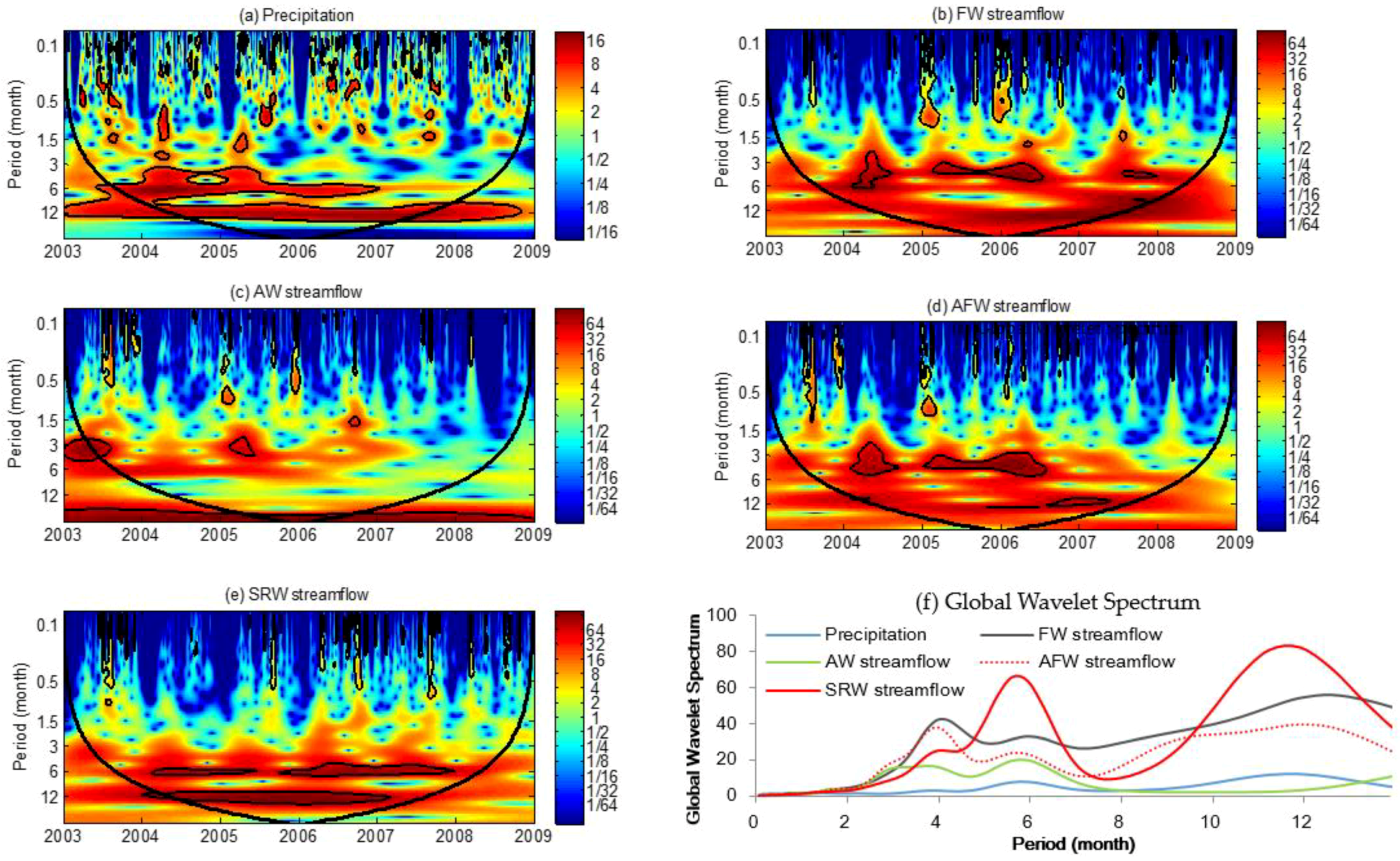
3.2.2. The CWT Results of Daily Precipitation and Streamflow

The CWT result of the daily precipitation is shown in Figure 3a, and the CWT results of FW, AW, AFW and SRW daily streamflow are shown in Figure 3b–e, respectively. Colors indicate the strength of the wavelet spectral power, with red areas indicating higher values and blue areas indicating smaller values. The 5% significance level against red noise calculated using Monte Carlo method is indicated by the thin black contours, and the thick black line separated the edge affected spectral power which could be underestimated. The five series have, respectively, first-order autoregressive (AR1) coefficient with lag 1 of 0.27, 0.93, 0.96, 0.90 and 0.91, which is used to assess the statistical significance of the wavelet power [38]. The x-axis shows the time of six years from 2003 to 2008, while y-axis shows the period in months. The GWS of CWT is shown in Figure 3f, which can provide the time average of the wavelet spectrum and permit an overall view of daily precipitation and streamflow [39].
For the CWT of precipitation (Figure 3a), two main time bands (0–3 months and 3–12 months) can be identified. For the CWTs of streamflow (Figure 3b–e), two main time bands from 0–2 months and 2–12 months can be identified. In the 0–3 months’ periods, fluctuation in precipitation are practically absent, whereas fluctuations in streamflow are absent in the 0–2 months’ period and significant in the 2–3 months’ period. In the 3–12 months’ period, both precipitation and streamflow wavelet spectrum increase, though higher for streamflow. During March-June, we observe notable intensity at 0–2 months’ period in FW and AW streamflow CWTs. The notable intensity during this period is coinciding with the snowmelt events. During July to September, we observe notable intensity at 0–2 months’ period in FW and AW streamflow CWTs, coinciding with the rainfall events. Similar results were found in AFW and SRW, except that during the 1-year’ s period CWT spectral power of SRW streamflow was more significant than that of AFW streamflow. For the FW streamflow CWT, a substantial intensity for the 3–12 months’ period was observed during 2003–2008. While for the AW streamflow CWT, a substantial intensity for the 3-6-months’ period was observed during 2003–2008. During 7–12 months’ period, the CWT spectral power for the AW streamflow was much lower than that for FW streamflow. These results are in accordance with the GWS results. The GWS of FW streamflow shows obvious peaks at 3–4, 6 and 12 months’ period. Similar results were found for AFW and SRW. However, for the CWT of AW streamflow, the substantial intensity for the 3–6 months’ period was found during 2003–2006. Its GWS shows obvious peaks at 3–4 and 6 months’ period, while annual periodicity was not found. The GWS of AFW streamflow lines between FW and AW, while the GWS of SRW streamflow shows much higher peaks at 6 and 12 months’ period. The GWS of AFW streamflow is aligned with that of FW at 3–4, 6 and 12 months’ period, and AW at 3–4 and 6 months’ period. It might therefore be used to obtain information about coupled land use and topography effect on streamflow variability and response to precipitation.

3.2.3. The XWT of Precipitation and Streamflow

The XWTs of precipitation and streamflow of FW, AW, AFW and SRW are shown in Figure 4a–d), respectively. The XWT GWS for the four pairs is shown in Figure 4e. It is observed that precipitation and streamflow show higher common power from 3 to 12 months’ period than 0 to 3 months’ period in FW (Figure 4a), with peaks at 4, 6 and 12 months’ period (Figure 4e). However, precipitation and streamflow XWT has higher common power from 3 to 6 months’ period than 6–12 months’ period in AW (Figure 4b), with peaks at 4 and 6 months’ period (Figure 4e). The precipitation and streamflow XWT spectral power of AW is much lower and not significant compared with that of FW during the 12 months’ period. Precipitation and streamflow XWT show similar patterns in the AFW and SRW, which shows higher common power from 3 to 12 months’ period than 0 to 3 months’ period, with peaks at 4, 6 and 12 months’ period. The common power at 6 and 12 months’ periods in SRW are the highest than that in other sites, which could be due to the highest total amount of EXT in SRW. The XWT of precipitation and streamflow in AFW/SRW has a similar magnitude with that in FW for 0–12 months’ period (see also the corresponding XWT GWS), whereas the XWT of precipitation and streamflow in AFW/SRW only shows a closer relationship with AW for the 0–8 months’ periods.

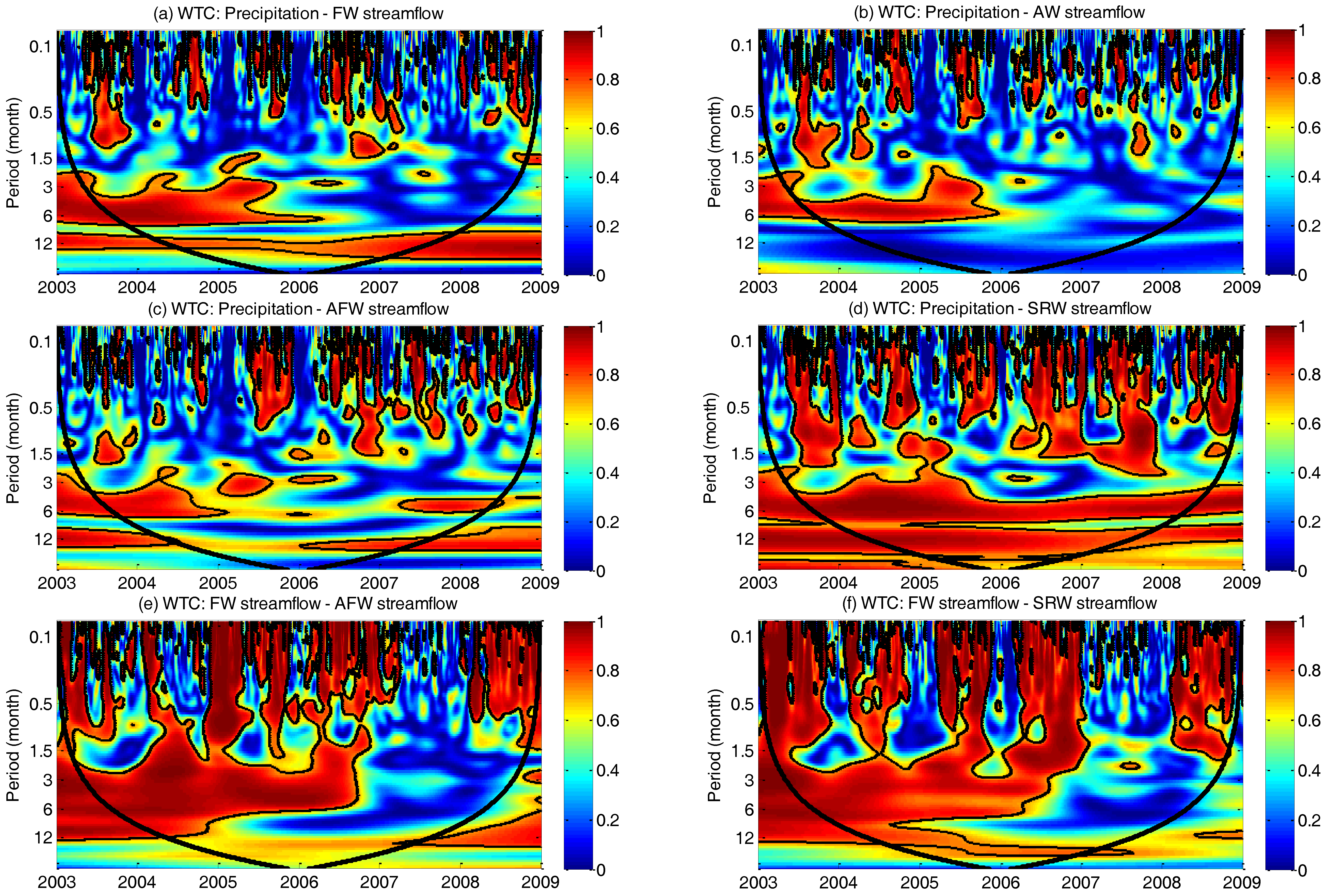
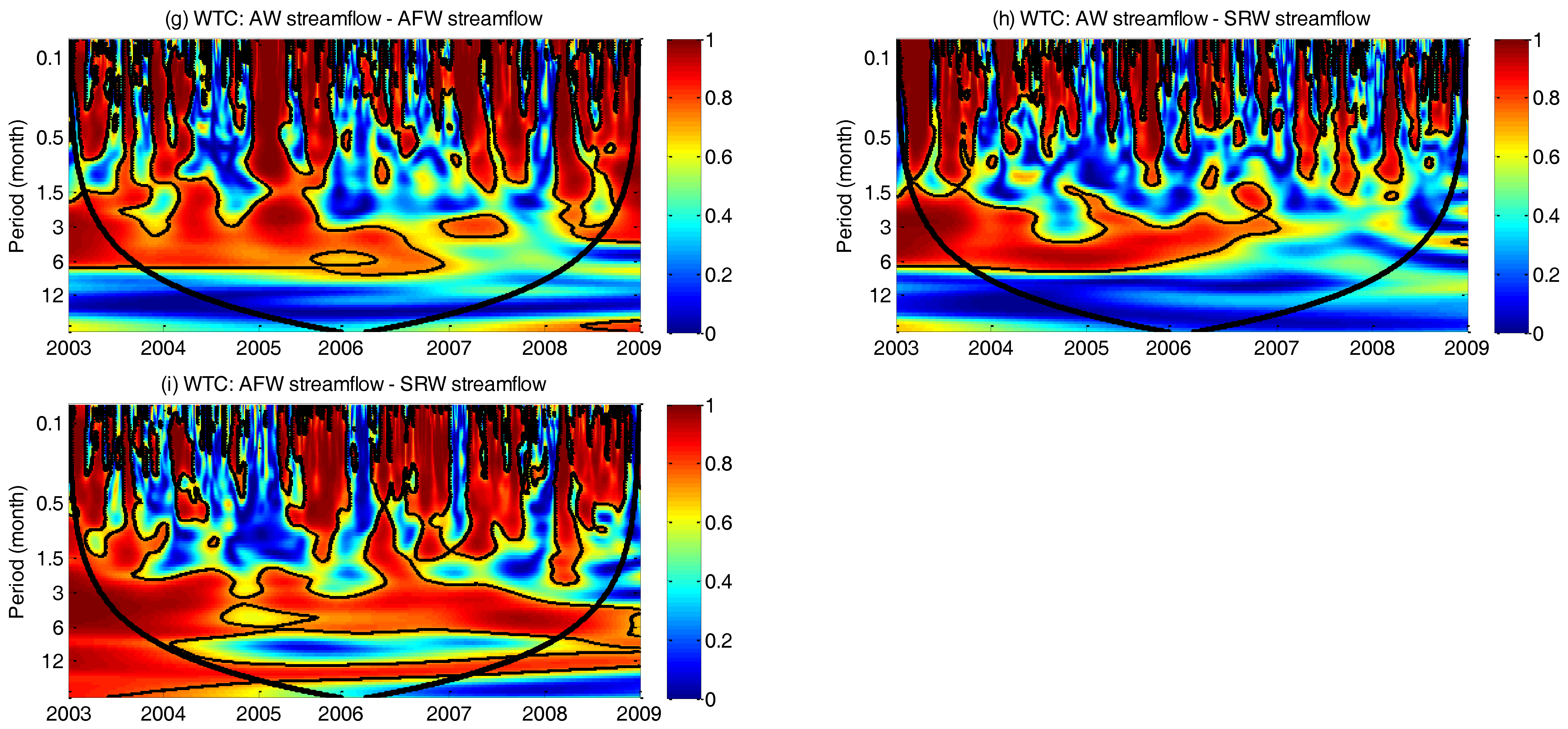
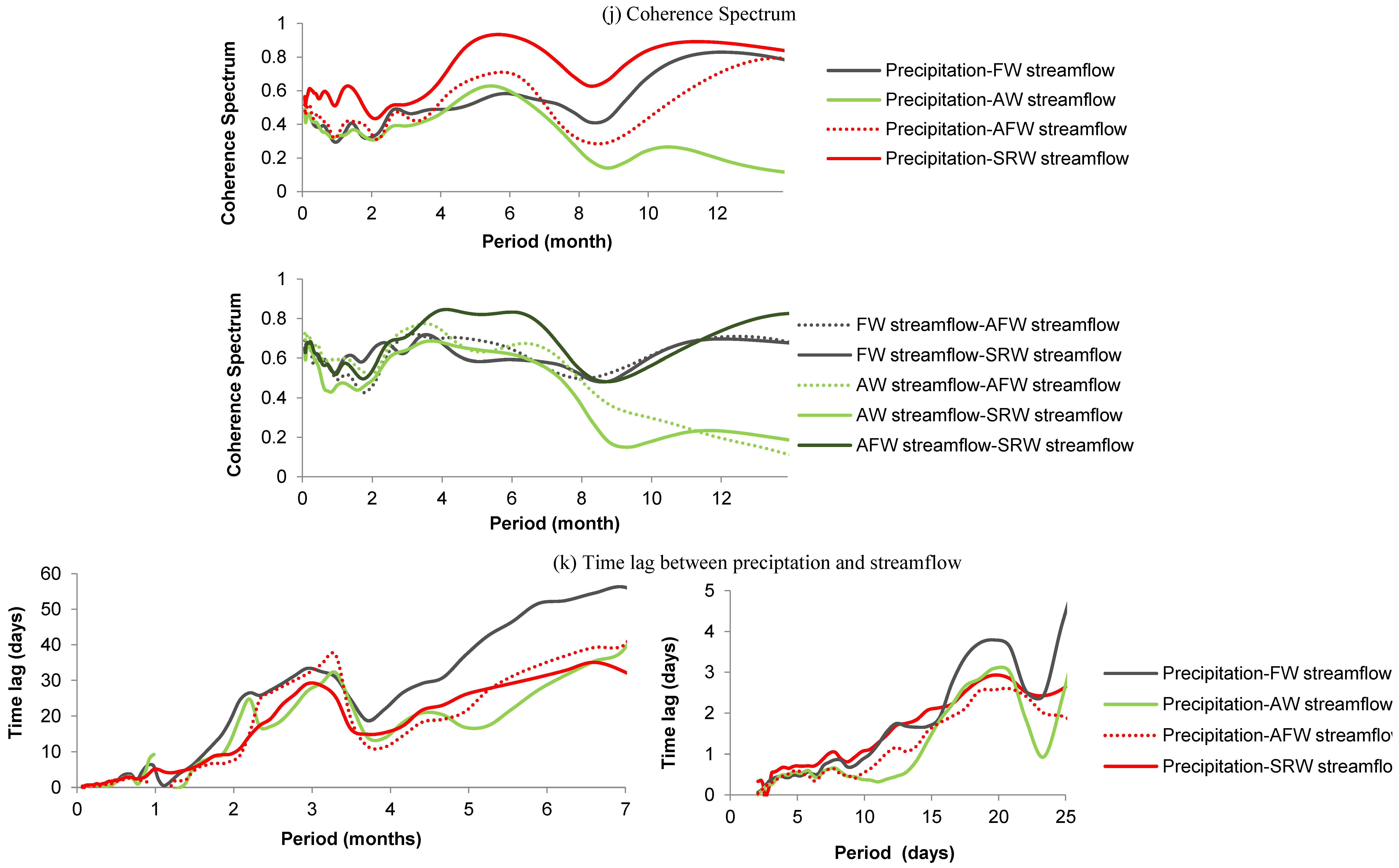
3.2.4. WTC of Precipitation and Streamflow and Time Lag

Figure 5a–d indicate the relationships between precipitation and streamflow in the four watersheds using WTC, Figure 5e–i indicate the relationships between streamflow of different watersheds using WTC, and the WTC GWS is shown in Figure 5j. For the 0–4 months’ period, the average WTC is greater than 0.4 for FW, AW and AFW, while it is higher than 0.5 for SRW. During the 0–1.5 months’ period for year 2007, there is a loss of coherence between precipitation and streamflow in FW compared with that in AW. During the 4–7 months’ period, there is an increase of coherence, the average WTC is greater than 0.5 for FW, AW and AFW, while SRW had the higher coherence of 0.7 on average. During the 7–9 months’ period, there is a decrease of coherence for all series. During the 9–12 months’ period, there is a complete loss of coherence for AW, while the average WTC is 0.7 for FW, 0.6 for AFW, and 0.8 for SRW. For all periods the covariance between precipitation and streamflow in SRW is always much higher than that in AFW.
As Figure 5e–i illustrates, for the relationship between streamflow of different watersheds using WTC, the FW-AFW and FW-SRW streamflow (Figure 5e,f) show higher covariance than AW-AFW and AW-SRW streamflow (Figure 5g,h) during the 0–12 months’ period from 2003–2008 except 2007. In year 2007, AW-AFW and AW-SRW streamflow shows higher covariance than FW-AFW and FW-SRW streamflow during the 0–6 months’ period. The AFW-SRW streamflow also shows high covariance during the 0–12 months’ period from 2003–2008 (Figure 5i). Overall, the average WTC is 0.6 for FW-AFW, FW-SRW, and AFW-SRW streamflow during the 0–12 months’ period and for AW-AFW, and AW-SRW streamflow during the 0–7 months’ period. There is a loss of covariance between AW-AFW streamflow and AW-SRW streamflow during the 7–12 months’ period. The WTC of FW-AFW streamflow and AW-AFW streamflow are similar with FW-SRW streamflow and AW-SRW streamflow, respectively. The covariance between streamflow in SRW and AFW is as high as 0.6 for the 0–4 months’ period and 0.8 for the 4–6 and 12 months’ period. Therefore, the SRW streamflow appears similar trends to that of AFW streamflow.
Time lag between the precipitation and streamflow in the four watersheds during each period is shown in Figure 5k. By analyzing the time lag between the precipitation and streamflow in the four watersheds for the 0–1 month’s period, it is found that there is a 0.5 day delay during the 2–10 days’ period, and an increased 3 days delay during the 10 days–1 month’s period. By comparing the time delays of streamflow response to precipitation in FW and AW, it can be seen that they are similar during the 2–10 days’ period at the two watersheds, and time lag in AW is only about 0.5 day shorter than that that in FW. Looking at the time delay of streamflow response to precipitation for the 1–3 months’ period, we can see for the four watersheds, time lag all increases from 3 days to 40 days. The time delay in AW is about 2 days shorter than that in FW for the 1–2 months’ period and 10 days shorter than that in FW for the 2–3 months’ period. There are decreases of time lag at 3–4 months’ period, and time delays are similar for all the watersheds. Then the time delay increase again until the 7 months’ period for all the watersheds. During the 4–7 months’ period, the time delay increased from 15 days to 40 days in AW, while it increased from 20 days to 55 days in FW. The time delay in AW is about 15 days shorter than that in FW. Comparing the time delay between precipitation and streamflow in AFW and SRW during the 2 days–7 months’ period, it can be found that both of them are similar and showed the similar values with those in FW and AW. Generally, during 7–9 months’ period, there are sharp changes of time delay for all the comparisons, and therefore, it cannot permit any other firm conclusions. During 10–12 months’ period, precipitation and streamflow varied synchronously in FW, AFW and SRW except AW.

4. Discussion

4.1. Coupled Effects of Land Use and Topography on Streamflow Variability

For the annual and monthly precipitation variability of all the watersheds, the CvPA is 0.22 and CvPmo is 0.83 (Table 2). In the Shibetsu River Watershed, precipitation exhibits low annual variability and distinct dry/wet seasons in a year. Similar CvPmo values were found in other northern watersheds, such as HJ Andrews, Wolf Creek, and KryckIan, as reported by Carey et al. [31]. Continuous wavelet analysis results show that precipitation (rainfall and snowmelt) variability of Shibetsu River Watershed are characterized by 1-year, 0.5-year periods (Figure 3), while only 1 year period was found in the area without snowfall and snowmelt as reported in other studies [40]. The lesser intensity of CWT for precipitation compared with streamflow is because precipitation is less structured than streamflow (Figure 3).
Streamflow variability was assessed in three parts for the four watersheds with different land use and topography interactions. Firstly, magnitude of streamflow components (direct runoff, baseflow, and total streamflow) was analyzed. Among the four watersheds, FW showed the highest surface runoff, baseflow, and total streamflow, while AW showed the lowest. These results indicated that despite higher surface soil hydraulic conductivity in the forests than the pasture, coupled forest and steep topography produced more surface runoff compared with coupled pasture and flat topography. It might be because forested soil has stronger and more persistent water repellency due to the high organic matter contents under dry conditions [41]. In addition, the steep slope gradients of the forest as compared to the pasture could have played a role, which results in a shorter time for water remaining on the soil because of the gravity effect lower water storage capacity on steep slopes [42]. However, it should be noted that the subsurface flow and total streamflow in FW were both higher than AW. It could be due to forest areas might be where external groundwater flows into Shibetsu River Watershed indicated by the presences of springs in steep forest areas according to the field investigations [24], thus FW received more EXT and had higher baseflow and total streamflow. In the absence of a meteorological station in the forest, the precipitation could be higher and evapotranspiration could be lower in the forest, which might result in the higher surface runoff and baseflow in FW [43]. These findings contradict with previous study that pasture showed higher annual streamflow through high baseflow in comparison to the forested watershed due to lower interception and evapotranspiration of pasture land [44]. For most events at both AW and FW watersheds, vertical soil water movement in volcanic soils and bedrocks can produce high subsurface flow. With the increase of soil antecedent wetness, subsurface flow might increase correspondingly, thus, groundwater flow might have contributed more to the streamflow [45,46]. Streamflow in the four watersheds were all dominated by subsurface sources, which might because volcanic soil has higher infiltration rate than average rainfall intensity [23].
Secondly, streamflow variability in the four watersheds was determined by analyzing the streamflow variability (coefficient of variation at annual (CvQA) and monthly scale (CvQmo)). Annual streamflow varies slightly among the watersheds (Table 2). The variability of annual streamflow exhibits similar trend with annual precipitation for all the watersheds. Similar to CvQA, the Cv of monthly streamflow (CvQrno) represents monthly variability of streamflow. The site FW has higher CvQrno value compared with AW, indicating that coupled forest land use and steep topography has higher monthly streamflow variability than coupled pasture land use and flat topography.
Thirdly, based on CWT, main variability mode over time of the four watersheds were determined. The streamflow of FW shows similar variability with precipitation, which is characterized by 3–4 months, 6 months, and 1-year periods. However, the 1-year period was not found in AW streamflow (Figure 3). It could be due to that the lower slope gradient resulted in a smaller subsurface water storage capacity. Thus, baseflow during snowmelt season (March–May) showed similar magnitude with that during the main rainfall season (July–September) (Figure 2). This was also reported by other studies, which reported that coupled pasture land use and flat topography tended to have less capacity to store groundwater [23]. The AFW and SRW streamflow show similar variability with precipitation, which is characterized by 1-year, 6 months, 3–4 months’ periods. The 3–4 months and 6 months’ periods could be explained by the mixed effects of pasture/flat topography and forest/steep topography, while 1-year period is due to the effects of coupled forest/steep topography. The CWT GWS of AFW is smaller than that of FW and higher than that of AW (Figure 3f) for all the periods, which also indicates double effects of coupled pasture/flat topography and coupled forest/steep topography. The less intensity of CWT and smaller CWT GWS of streamflow in AW could be due to AW streamflow is less influenced by its preceding states, thus, less structured than FW streamflow. (Figure 2 and Figure 3).

4.2. Coupled Effects of Land Use and Topography on Streamflow Response to Precipitation

The streamflow response to precipitation was analyzed in four parts for the four watersheds with different land use and topography combinations. Firstly, how closely precipitation and streamflow is correlated was analyzed with the ratio of streamflow and precipitation Cv at annual (CvQA/CvPA) and monthly scale (CvQrno/CvPrno). Secondly, when and which periods that precipitation and streamflow has high common spectral power were analyzed using XWT. Thirdly, when and which periods the precipitation and streamflow co-variation were analyzed using WTC. Lastly, the delay between the precipitation and streamflow was analyzed based on XWT time lag.
Values of CvQA/CvPA and CvQrno/CvPrno close to 1 and higher cor(QA, PA) and cor(Qmo, Pmo) indicate a greater synchronicity in precipitation and streamflow at annual and monthly scale. Precipitation and streamflow characteristics showed that FW has greater synchronicity in precipitation and streamflow at annual and monthly scale than AW (Table 2). This finding is consistent with Carey et al. [31], which reported that catchments with gentle topography have lower cor(Qmo, Pmo) than catchments with steep topography. The statistical result is also consistent with XWT and WTC analysis in this study. The XWT analysis shows that precipitation and streamflow show high common spectral power from 3 to 12 months periods in FW, while only show high common spectral power from 3 to 6 months periods in AW. The WTC analysis shows that coherence is higher from 6–12 months periods in FW than AW. The FW has greater synchronicity in precipitation and streamflow than AW for the longer periods of 3–12 months (Figure 5), which could be due to higher rainfall interception and enhanced water storage capacity in forest. Besides, steep topography usually has more permeable bedrock substrates, thus, it could have higher subsurface water storage capacity and slower drainage [47]. However, the WTC analysis results indicated that precipitation and streamflow in FW shows lower coherency than that in AW in year 2007 (Figure 5), which could be due to lower rainfall interception and lower surface soil infiltration capacity in pasture land under wet antecedent conditions caused by large precipitation in years 2006 and 2007. The coupling at shorter periods occurred during wet periods when the pasture was responsive and water storage deficits were small in flat topography [23]).
Compared with FW, AW showed the shortest time lags between precipitation and streamflow during the 0–7 months period, indicating coupled pasture and flat topography has quicker streamflow response to precipitation. This is in accordance with previous study conducted by Jiang et al. [25] in the same watershed, which reported that the streamflow in AW peaked before FW during the snowmelt season in years 2004 and 2005, and storm events in 7 September 2004. This was also consistent with previous study in other sites [23], which reported that pasture watershed with mean slope of 18° showed shorter time lag than forest watershed with mean slope above 30° during a 6-week wetting up cycle. They also reported that the lower rainfall interception and soil hydraulic conductivity due to compaction by grazing in pasture could explain streamflow’s quicker response to precipitation in small periods. The watershed with steep topography usually has more permeable bedrock substrates, thus, it could have higher water storage capacity than watershed with gentle topography. Therefore, watershed with steep topography could show lower streamflow responsiveness to precipitation [47]. In addition, although the groundwater flow was the main components of baseflow in the agricultural pasture watershed, it might be delivered from a shallower subsurface compartment, thus, show quicker streamflow responsiveness, as compared to forested watershed [23]. Effect of watershed size on the time lag between precipitation and streamflow could be eliminated in this study because time lag in SRW was smaller than that in FW in this study. Results of this study indicated that coupled land use and topography controls on response of streamflow to precipitation.
Coupled effects of land use and topography on streamflow variability and responsiveness were assessed in this study. Some other factors, such as climate, soil, geology, and storage capacity, may also influence the hydrologic responsiveness. Quantifying the effects of all these factors or an individual factor on streamflow is still a challenge. The statistical methods, distributed rainfall-runoff models or physically-based hydrologic models combining scenarios analysis could be adopted to quantify the effects of land use and/or topography on streamflow [48,49]. Future studies should adopt more methods to quantify the effects of an individual factor and integrated factors on hydrologic processes.

5. Conclusions

In this study, we explored the effects of land use and topography interactions on streamflow in three headwater watersheds in Shibetsu River Watershed, Hokkaido, Japan. Our results showed that the integrated land use and topography probably regulated the streamflow components, variability and responsiveness to precipitation. Coupled forest and steep topography can produce higher surface runoff than coupled pasture and flat topography due to forested surface soil water repellency and steep slope. In addition, watershed with coupled forest and steep topography showed the higher baseflow and total streamflow which might be due to lower evapotranspiration, higher external groundwater source and higher precipitation in the forested areas. The watershed with coupled forest and steep topography showed higher coherence between precipitation and streamflow except at times under high antecedent wetness conditions when the lower soil hydraulic conductivity and water storage deficit in pasture might play the role. Watershed with pasture and flat topography showed quicker streamflow response to precipitation, which might be due to lower rainfall interception, reduced soil hydraulic conductivity, and lower storage capacity. Combinations of different land uses and topography cause different streamflow generation sources and processes. Our results showed that understanding the effects of land use and topography on streamflow could benefit the surface water source regulation, modulation of streamflow responses to rainfall, and flood control. In future studies, more work is needed to quantify and separate the effect of climate, topography, soil and vegetation influences.

Author Contributions

C.W. conceived this study, analyzed the data and wrote the paper; D.J. performed the calculations and provided the land use and topographic maps; S.Shang, Y.H., S.Sauvage and J.-M.S.-P. provided feedback on the drafts and the revised versions of the paper; K.K. and R.H. provided the data.

Acknowledgments

This work was supported by the National Natural Science Foundation of China (No. 51609084), Open Research Fund Program of State Key Laboratory of Hydroscience and Engineering, Tsinghua University (sklhse-2016-A-01), the ‘948′ Project of Ministry of Water Resources of China (Grant No. 201328), the JSPS Grants-in-aid for Scientific Research (No. 26511001). The authors also sincerely thank, F. Salerno at Water Research Institute, National Research Council (IRSA-CNR), Località Occhiate, Brugherio, Milan, Italy, for his valuable suggestions on wavelet analysis methods. The authors would also like to thank the editor and all the reviewers for their insightful comments and constructive suggestions.

Conflicts of Interest

The authors declare no conflicts of interest.

References

  1. Price, K. Effects of watershed topography, soils, land use, and climate on baseflow hydrology in humid regions: A review. Prog. Phys. Geogr. 2011, 35, 465–492. [Google Scholar] [CrossRef]
  2. Price, K.; Jackson, C.R.; Parker, A.J.; Reitan, T.; Dowd, J.; Cyterski, M. Effects of watershed land use and geomorphology on stream low flows during severe drought conditions in the southern Blue Ridge Mountains, Georgia and North Carolina, USA. Water Resour. Res. 2011, 47, W02516. [Google Scholar] [CrossRef]
  3. Chen, X.; Cheng, Q.; Chen, Y.D.; Smettem, K.; Xu, C. Simulating the integrated effects of topography and soil properties on runoff generation in hilly forested catchments, South China. Hydrol. Process. 2010, 24, 714–725. [Google Scholar] [CrossRef]
  4. Strauch, A.M.; MacKenzie, R.A.; Giardina, C.P.; Bruland, G.L. Climate driven changes to rainfall and streamflow patterns in a model tropical island hydrological system. J. Hydrol. 2015, 523, 160–169. [Google Scholar] [CrossRef]
  5. Pokhrel, Y.; Burbano, M.; Roush, J.; Kang, H.; Sridhar, V.; Hyndman, D.W. A Review of the Integrated Effects of Changing Climate, Land Use, and Dams on Mekong River Hydrology. Water 2018, 10, 266. [Google Scholar] [CrossRef]
  6. Foley, J.A.; DeFries, R.; Asner, G.P.; Barford, C.; Bonan, G.; Carpenter, S.R.; Chapin, F.S.; Coe, M.T.; Daily, G.C.; Gibbs, H.K.; et al. Global Consequences of Land Use. Science 2005, 22, 570–574. [Google Scholar] [CrossRef] [PubMed]
  7. Li, J.; Liu, D.; Wang, T.; Li, Y.; Wang, S.; Yang, Y.; Wang, X.; Guo, H.; Peng, S.; Ding, J.; et al. Grassland restoration reduces water yield in the headstream region of Yangtze River. Sci. Rep. 2017, 7, 2162. [Google Scholar] [CrossRef] [PubMed]
  8. Roa-García, M.C.; Brown, S.; Schreier, H.; Lavkulich, L.M. The role of land use and soils in regulating water flow in small headwater catchments of the Andes. Water Resour. Res. 2011, 47, W05510. [Google Scholar] [CrossRef]
  9. Germer, S.; Neill, C.; Vetter, T.; Chaves, J.; Krusche, A.V.; Elsenbeer, H. Implications of long-term land-use change for the hydrology and solute budgets of small catchments in Amazonia. J. Hydrol. 2009, 364, 349–363. [Google Scholar] [CrossRef]
  10. Chhabra, A.; Geist, H.; Houghton, R.A.; Haberl, H.; Braimoh, A.K.; Vlek, P.; Patz, J.; Xu, J.C.; Ramankutty, N.; Coomes, O.; et al. Multiple impacts of land use/cover change. In Land-Use and Land-Cover Change: Local Processes and Global Impacts; Lambin, E.F., Geist, H.J., Eds.; Springer: Berlin, Germany, 2006; pp. 71–116. [Google Scholar]
  11. Farley, K.A.; Jobbagy, E.G.; Jackson, R.B. Effects of afforestation on water yield: A global synthesis with implications for policy. Glob. Ch. Biol. 2005, 11, 1565–1576. [Google Scholar] [CrossRef]
  12. Wang, R.; Kalin, L.; Kuang, W.; Tian, H. Individual and combined effects of land use/cover and climate change on Wolf Bay watershed streamflow in southern Alabama. Hydrol. Process. 2014, 28, 5530–5546. [Google Scholar] [CrossRef]
  13. Dias, L.C.P.; Macedo, M.N.; Costa, M.H.; Coe, M.T.; Neill, C. Effects of land cover change on evapotranspiration and streamflow of small catchments in the Upper Xingu River Basin, Central Brazil. J. Hydrol. Reg. Stud. 2015, 4, 108–122. [Google Scholar] [CrossRef]
  14. Yao, Y.; Wang, X.; Zeng, Z.; Liu, Y.; Peng, S.; Zhu, Z.; Piao, S. The effect of afforestation on soil moisture content in Northeastern China. PLoS ONE 2016, 11, e0160776. [Google Scholar] [CrossRef] [PubMed]
  15. Bruijnzeel, L.A. Hydrological functions of tropical forests: Not seeing the soil for the trees? Agric. Ecosyst. Environ. 2004, 104, 185–228. [Google Scholar]
  16. Ma, X.; Xu, J.; Luo, Y.; Aggarwal, S.P.; Li, J. Responses of hydrological processes to land-cover and climate changes in Kejie Watershed, South-West China. Hydrol. Process. 2009, 23, 1179–1191. [Google Scholar] [CrossRef]
  17. Beven, K.; Kirkby, M.J. A physically-based, variable contributing area model of basin hydrology. Hydrol. Sci. Bull. 1979, 24, 43–69. [Google Scholar]
  18. Tetzlaff, D.; Seibert, J.; McGuire, K.J.; Laudon, H.; Burn, D.A.; Dunn, S.M.; Soulsby, C. How does landscape structure influence catchment transit time across different geomorphic provinces? Hydrol. Process. 2009, 23, 945–953. [Google Scholar] [CrossRef]
  19. Moraes, J.M.; Schuler, A.E.; Dunne, T.; Figueiredo, R.O.; Victoria, R.L. Water storage and runoff processes in plinthic soils under forest and pasture in Eastern Amazonia. Hydrol. Process. 2006, 20, 2509–2526. [Google Scholar] [CrossRef]
  20. Soares-Filho, B.S.; Nepstad, D.C.; Curran, L.M.; Cerqueira, G.C.; Garcia, R.A.; Ramos, C.A.; Voll, E.; McDonald, A.; Lefebvre, P.; Schlesinge, P. Modelling conservation in the Amazon Basin. Nature 2006, 440, 520–523. [Google Scholar] [CrossRef] [PubMed]
  21. Muñoz-Piña, C.; Guevara, A.; Torres, J.M.; Braña, J. Paying for the hydrological services of Mexico’s forests: Analysis, negotiations and results. Ecol. Econ. 2008, 65, 725–736. [Google Scholar] [CrossRef]
  22. Barona, E.; Ramankutty, N.; Hyman, G.; Coomes, O.T. The role of pasture and soybean in deforestation of the Brazilian Amazon. Environ. Res. Lett. 2010, 5, 1–9. [Google Scholar] [CrossRef]
  23. Muñoz-Villers, L.E.; McDonnell, J.J. Land use change effects on runoff generation in a humid tropical montane cloud forest region. Hydrol. Earth Syst. Sci. 2013, 17, 3543–3560. [Google Scholar] [CrossRef]
  24. Jiang, R.; Li, Y.; Wang, Q.; Kuramochi, K.; Hayakawa, A.; Woli, K.P.; Hatano, R. Modeling the water balance processes for understanding the components of river discharge in a non-conservative watershed. Trans. ASABE 2011, 54, 2171–2218. [Google Scholar] [CrossRef]
  25. Jiang, R.; Woli, K.P.; Kuramochi, K.; Hayakawa, A.; Shimizu, M.; Hatano, R. Coupled control of land use and topography on nitrate-nitrogen dynamics in three adjacent watersheds. Catena 2012, 97, 1–11. [Google Scholar] [CrossRef]
  26. Tachibana, H.; Nasu, Y. Measurement of runoff. In Water Analysis; Kagaku Dojin: Kyoto, Japan, 2003; pp. 362–370. [Google Scholar]
  27. Motoyama, H. Simulation of seasonal snowcover based on air temperature and precipitation. J. Appl. Meteorol. 1990, 29, 1104–1110. [Google Scholar] [CrossRef]
  28. Reinel, S.-A.; Joe, R. M.; William, J.M. Effects of temperature and precipitation on snowpack variability in the Central Rocky Mountains as a function of elevation. Geophys. Res. Lett. 2015, 42, 4429–4438. [Google Scholar]
  29. Arnold, J.; Allen, P. Automated methods for estimating baseflow and ground water recharge from streamflow records. J. Am. Water Resour. Assoc. 1999, 35, 411–424. [Google Scholar] [CrossRef]
  30. Nathan, R.J.; MaMahon, T.A. Evaluation of automated techniques for baseflow and recession analysis. Water Resour. Res. 1990, 26, 1465–1473. [Google Scholar] [CrossRef]
  31. Carey, S.K.; Tetzlaff, D.; Seibert, J.; Soulsby, C.; Buttle, J.; Laudon, H.; McDonnell, J.; McGuire, K.; Caissie, D.; Shanley, J.; et al. Inter-comparison of hydro-climatic regimes across northern catchments: Synchronicity, resistance and resilience. Hydrol. Process. 2010, 24, 3591–3602. [Google Scholar] [CrossRef]
  32. Daubechies, I. Ten Lectures on Wavelets; Society for Industrial and Applied Mathematics: Philadelphia, PA, USA, 1992; p. 357. [Google Scholar]
  33. Meyer, Y. Ondelettes et Opérateurs I; Hermann: Paris, France, 1989; p. 215. (In French) [Google Scholar]
  34. Torrence, C.; Compo, G.P. A practical guide to wavelet analysis. Bull. Am. Meteorol. Soc. 1998, 79, 61–78. [Google Scholar] [CrossRef]
  35. Torrence, C.; Webster, P.J. Interdecadal changes in the ESNO-monsoon system. J. Clim. 1999, 12, 2679–2690. [Google Scholar] [CrossRef]
  36. Grinsted, A.; Moore, J.; Jevrejeva, S. Application of the cross wavelet transform and wavelet coherence to geophysical time series. Nonlinear Process. Geophys. 2004, 11, 561–566. [Google Scholar] [CrossRef]
  37. Wang, C.; Jiang, R.; Mao, X.; Sauvage, S.; Sánchez-Pérez, J.M.; Woli, K.P.; Kuramochi, K.; Hayakawa, A.; Hatano, R. Estimating sediment and particulate organic nitrogen and particulate organic phosphorous yields from a volcanic watershed characterized by forest and agriculture using SWAT model. Annales Limnol. Int. J. Limnol. 2015, 51, 23–35. [Google Scholar] [CrossRef]
  38. Allen, M.R.; Smith, L.A. Monte Carlo SSA: Detecting irregular oscillations in the presence of coloured noise. J. Clim. 1996, 9, 3373–3404. [Google Scholar] [CrossRef]
  39. Kestin, T.A.; Karoly, D.J.; Yano, J.I.; Rayner, N.A. Time-frequency variability of ENSO and stochastic simulations. J. Clim. 1998, 11, 2258–2272. [Google Scholar] [CrossRef]
  40. Salerno, F.; Tartari, G. A coupled approach of surface hydrological modelling and Wavelet Analysis for understanding the baseflow components of river discharge in karst environments. J. Hydrol. 2009, 376, 295–306. [Google Scholar] [CrossRef]
  41. Ellis, A.; Ramirez, C.; Mac Donald, R.H. Wetting capacity distribution in aggregates from soils with a different management. J. Food Agric. Environ. 2003, 1, 229–233. [Google Scholar]
  42. Khan, M.N.; Gong, Y.; Hu, T.; Lal, R.; Zheng, J.; Justine, M.F.; Azhar, M.; Che, M.; Zhang, H. Effect of slope, rainfall intensity and mulch on erosion and infiltration under simulated rain on purple soil of South-Western Sichuan Province, China. Water 2016, 8, 528. [Google Scholar] [CrossRef]
  43. Sawano, S.; Komatsu, H.; Suzuki, M. Differences in annual precipitation amounts between forested area, agricultural area, and urban area in Japan. J. Jpn. Soc. Hydrol. W. Resour. 2005, 18, 435–440. [Google Scholar] [CrossRef]
  44. Muñoz-Villers, L.E.; McDonnell, J.J. Runoff generation in a steep, tropical montane cloud forest catchment on permeable volcanic substrate. Water Resour. Res. 2012, 48, W09528. [Google Scholar] [CrossRef]
  45. Sidle, R.C. Stormflow generation in forest headwater catchments: A hydrogeomorphic approach. For. Snow Landsc. Res. 2006, 80, 115–128. [Google Scholar]
  46. Sidle, R.C.; Tsuboyama, Y.; Noguchi, S.; Hosoda, I.; Fujieda, M.; Shimizu, T. Stormflow generation in steep forested headwaters: A linked hydrogeomorphic paradigm. Hydrol. Process. 2000, 14, 369–385. [Google Scholar] [CrossRef]
  47. Sayama, T.; McDonnell, J.J.; Dhakal, A.; Sullivan, K. How much water can a watershed store? Hydrol. Process. 2011, 25, 3899–3908. [Google Scholar] [CrossRef]
  48. Luo, P.; He, B.; Duan, W.; Takara, K.; Nover, D. Impact assessment of rainfall scenarios and land-use change on hydrologic response using synthetic Area IDF curves. J. Flood Risk Manag. 2018, 11, S84–S97. [Google Scholar] [CrossRef]
  49. Luo, P.; Zhou, M.; Deng, H.; Lyu, J.; Cao, W.; Takara, K.; Nover, D.; Schladow, S.G. Impact of forest maintenance on water shortages: Hydrologic modeling and effects of climate change. Sci. Total Environ. 2018, 615, 1355–1363. [Google Scholar] [CrossRef]
Figure 1. Locations of the study sub-basins and land use and topography characteristics of the Shibetsu River Watershed (SRW).
Water 10 00633 g001
Figure 2. Daily precipitation and streamflow series: (a) precipitation, (b) components of FW streamflow, (c) components of AW streamflow, (d) components of AFW streamflow, and (e) components of SRW streamflow.
Water 10 00633 g002
Figure 3. Continuous wavelet transform (CWT) spectrum of (a) precipitation, (b) FW streamflow, (c) AW streamflow, (d) AFW streamflow, and (e) SRW streamflow, and (f) their Global Wavelet Spectrum. The wavelet power at each period is normalized by the Global Wavelet Spectrum (dimensionless).
Water 10 00633 g003
Figure 4. Cross Wavelet Transform (XWT) spectrums of (a) precipitation and FW streamflow, (b) precipitation and AW streamflow, (c) precipitation and AFW streamflow, and (d) precipitation and SRW streamflow, and (e) Cross Wavelet Spectrum for the four pairs.
Water 10 00633 g004
Figure 5. Wavelet Coherence (WTC) spectrum: (ad) precipitation and FW, AW, AFW streamflow, (ei) streamflow between FW-AFW, FW-SRW, AW- AFW, AW-SRW, and AFW-SRW, (j) the Coherence Spectrum for the above pairs, and (k) time lag between precipitation and streamflow.
Water 10 00633 g005aWater 10 00633 g005bWater 10 00633 g005c
Table 1. Land use and topographic characteristics for three headwater watersheds, i.e., agricultural watershed (AW), mixed agriculture-forested watershed (AFW), forested watershed (FW), and the whole Shibetsu River Watershed (SRW).
WatershedArea (km2)Land Use (%)Percentage of Areas with SlopesRelief Ratio
AgricultureForest0–10%>10%
AW14.373.523.597.62.40.0146
FW70.014.584.437.262.80.0553
AFW36.658.937.179.720.30.0362
SRW672.040.853.770.030.00.0173
Table 2. Contributions of streamflow in different watersheds.
WatershedSurface Flow
(mm day1)
Baseflow
(mm day1)
Baseflow Fraction
(%)
Total Streamflow
(mm day−1)
AW0.111.1384.11.24
FW0.562.9791.13.53
AFW0.381.8282.72.20
SRW0.382.4286.42.80
Table 3. Precipitation and streamflow characteristics in different watersheds.
WatershedCvPACvQACvQA/CvPAcor(QA, PA)CvPmoCvQmoCvQmo/CvPmocor(Qmo, Pmo)
AW0.220.281.270.090.830.340.410.01
FW0.220.261.180.750.830.650.780.06
AFW0.220.281.270.930.830.590.710.10
SRW0.220.261.180.940.830.540.650.21

