On Strong Nearshore Wind-Induced Currents in Flow-Through Gulfs: Variations on a Theme by Csanady

Abstract

Csanady’s (1973) model, used to explain the development of strong, wind-induced nearshore currents in long lakes, has been extended to explain the same phenomenon in flow-through semi-enclosed gulfs. As in the original theory, it is predicted that the depth-averaged velocities move with the wind in regions shallower than the characteristic depth and upwind in deeper parts of the basin. The characteristic depth in the modified theory, however, is shown to be larger than the characteristic depth of the original theory, which is the basin mean depth, by a parameter λ, which can be calculated using the wind stress, the cross-section area and the volumetric inflow into the gulf. The theory is further used to examine in detail the scaling of the flow and identify the dimensional parameters underlying the formulation of the Csanady model. By expanding in an appropriately-defined inverse, Rossby number, which can be made arbitrarily large for small times, it is shown that under the influence of the Coriolis force, the free surface assumes a characteristic S-like shape and the shorewise volume flux an M-like shape. It is suggested that the shorewise flux might be of interest in environmental applications. The predictions of both variations of the original model of Csanady have been illustrated by numerical simulations, in pertinent idealized geometries, and have been also used to explain salient features of the wind-induced circulation in the Gulf of Patras in Western Greece.

1. Introduction

A ubiquitous feature in simulations of wind-induced circulation in lakes of variable bathymetry is the strong nearshore currents that develop soon after the application of wind shear on the lake’s surface. This phenomenon is accompanied by a weak return flow (in the depth integrated sense), which seems to have been first reported by [1] and has been observed in many simulations ever since, up to recent ones. These currents are evident during the acceleration stage of flow and survive also at steady state. The phenomenon was explained by Csanady [2], who, in an insightful paper, developed a simple model (referred to as Csanady’s model) elucidating the phenomenon. That work, however, does not seem to have always been fully exploited (see, e.g., [3] or [4], where the justification for the strong nearshore currents is not dealt with explicitly). Csanady’s original model was developed for lakes, but the same phenomenon has been observed by [5] to occur also in simulations of wind-induced circulation in a flow-through, semi-enclosed gulf, namely the Gulf of Patras, in Western Greece. In this geometry, the wind-induced flow exhibits characteristics of both channel flow (e.g., non-zero cross-sectional flowrate, albeit with a very different streamwise velocity profile) and lake flow (e.g., free-surface setup).

Given the importance of strong nearshore wind-induced currents, we present below two variations of Csanady’s model. The first concerns flow-through gulfs and the second the effects of the Coriolis force. Both variations are illustrated with numerical simulations of wind-induced flow in idealized geometries and are also shown to be pertinent to the analysis of wind-induced flow in water bodies of natural geometry, such as the Gulf of Patras. Indeed, it is the need to interpret features of flow in natural geometries that has prompted the present analysis.

Csanady [2] developed his model from the linearized depth integrated flow equations. Herein, we expand the flow parameters in an $\epsilon =1/\mathcal{R}ℴ$ series, where $\mathcal{R}ℴ$ is a Rossby number, in order to quantify the influence of the Coriolis force. This makes it necessary to begin by scaling the full non-linear equations, so as to elucidate the influence of the other dimensionless flow and geometric parameters that enter the problem formulation.

Finally, in order to delineate the scope of the present work, it is worth noting that we do not view the following results as having prognostic value, since prognosis is nowadays best achieved with numerical simulation. Rather, these results are useful as diagnostic tools, elucidating features that appear in numerical simulations, and are not readily interpreted otherwise, as for example the S-shaped form of the free surface and the M-shaped shorewise flux, both in the cross-flow direction, under the influence of the Coriolis force.

2. The Non-Linear, Depth-Integrated Equations

2.1. The Geometry and the Equations

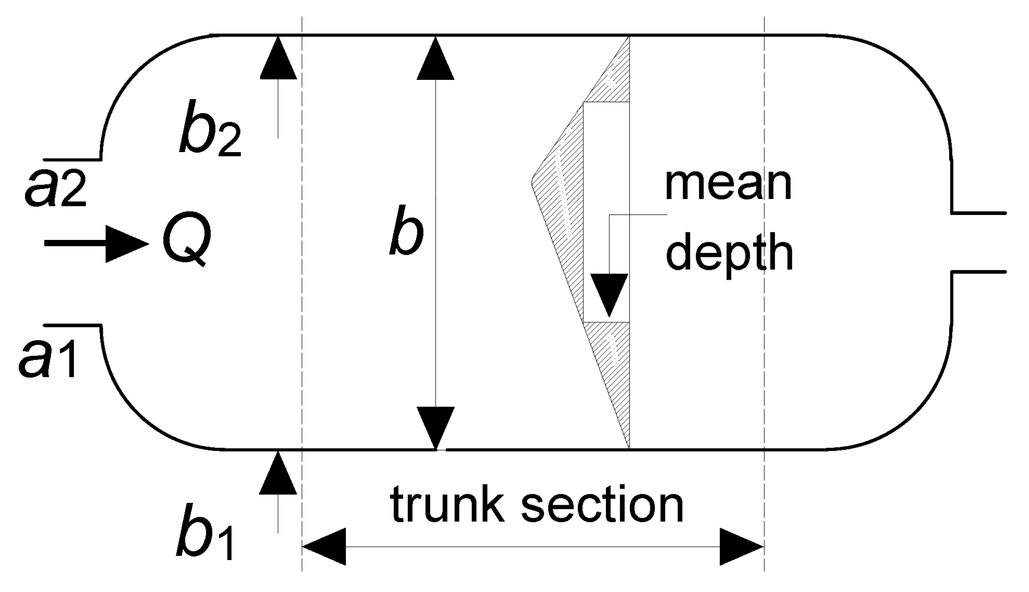
Csanady [2] considered the barotropic flow, which develops in a long lake with parallel shores and depth contours that curve at the end regions to create an enclosed geometry. An instance of such a geometry is depicted in Figure 1, only, in the original analysis, there is no inflow Q or outflow, since Csanady considered a lake. The parallel section of the lake he calls “a trunk”, and we keep his terminology herein. The non-linear, depth-integrated flow equations are (e.g., [6]):

$$\frac{\partial \eta }{\partial t}+\frac{\partial q_x}{\partial x}+\frac{\partial q_y}{\partial y}=0$$

(1)

$$\frac{\partial q_x}{\partial t}+\frac{\partial }{\partial x}\left(\frac{q_x^2}{\zeta }\right)+\frac{\partial }{\partial y}\left(\frac{q_x{q}_y}{\zeta }\right)=f{q}_y-g\zeta \frac{\partial \eta }{\partial x}+\frac{{\tau }_x}{\rho }-c_d\frac{q_x\left|q_x\right|}{{\zeta }^2}$$

(2)

$$\frac{\partial q_y}{\partial t}+\frac{\partial }{\partial x}\left(\frac{q_x{q}_y}{\zeta }\right)+\frac{\partial }{\partial y}\left(\frac{q_y^2}{\zeta }\right)=-f{q}_x-g\zeta \frac{\partial \eta }{\partial y}-c_d\frac{q_y\left|q_y\right|}{{\zeta }^2}$$

(3)

where $\eta$ is the deviation of the free-surface elevation from equilibrium (i.e., the mean water level), $\overrightarrow{q}=q_x\widehat{i}+q_y\widehat{j}$ the depth integrated flux, $q_x={{\displaystyle \int }}_{-h}^{\eta }udz$ and similarly for $q_y$, $h$ is the local depth and $\zeta =h+\eta$. Because of the assumed geometry, $h=h\left(y\right)$ in the trunk region, but $h=h\left(x,y\right)$ outside it. The width in the trunk is symbolized by $b$, the ordinates of the banks $b_1$ and $b_2$ (Figure 1), the wind shear stress, assumed constant over the water surface, by ${\tau }_x$, and the (constant) water density, by $\rho$. Below, when the pertinent external and intrinsic scales are used in order to render the equations nondimensional, $\eta$ will be considered to be small with respect to any reasonable measure of the cross-section depth $h$, such as the mean depth $\overline{h}$, which plays a special role in Csanady’s theory. It would have been more thorough to introduce an additional scale characterizing the minimum cross-section depth, such as $h_{min}$ because otherwise, if h is allowed to go to zero at the shores, artificial, fruitless difficulties arise. This would, however, overburden the presentation, and we prefer to tacitly assume the existence of such a scale.

2.2. The Dimensionless Equations and Dimensionless Parameters

In order to render the equations dimensionless, so as to bring out the dominant terms in a formal perturbation scheme, the external and intrinsic scales of the flow have to be used. Since we are to build around Csanady’s (1973) [2] solution, we use the scales compatible with it:

$$x~\mathcal{\ell },y~b,t~T,\eta ~\frac{{\tau }_x\mathcal{\ell }}{\rho g\overline{h}},q_x~\frac{{\tau }_{x}T}{\rho },q_y~\frac{{\tau }_{x}T}{\rho }\frac{b}{\mathcal{\ell }}$$

(4)

where $\mathcal{\ell }$ and $\overline{h}$ are scales of the length and trunk cross-sectional depth, respectively, $T$ is the time interval, no longer than the acceleration phase of the flow, and the other parameters have been defined above.

Using these scales, and letting the hat symbol $\widehat{\phantom{T}}$ denote the dimensionless quantities, the dimensionless equations appear as follows:

$$\mathcal{F}{𝓇}^2\frac{\partial \widehat{\eta }}{\partial \widehat{t}}+\frac{\partial {\widehat{q}}_x}{\partial \widehat{x}}+\frac{\partial {\widehat{q}}_y}{\partial \widehat{y}}=0$$

(5)

$$\begin{gathered} \frac{\partial {\widehat{q}}_x}{\partial \widehat{t}}+\frac{\mathcal{A}}{\mathcal{F}{𝓇}^2}\frac{\partial }{\partial \widehat{x}}\left(\frac{{\widehat{q}}_x^2}{\widehat{h}}\right)-\frac{{\mathcal{A}}^2}{\mathcal{F}{𝓇}^2}\frac{\partial }{\partial \widehat{x}}\left(\frac{{\widehat{q}}_x^2\widehat{\eta }}{{\widehat{h}}^2}\right)+\frac{\mathcal{A}}{\mathcal{F}{𝓇}^2}\frac{\partial }{\partial \widehat{y}}\left(\frac{{\widehat{q}}_x{\widehat{q}}_y}{\widehat{h}}\right)-\frac{{\mathcal{A}}^2}{\mathcal{F}{𝓇}^2}\frac{\partial }{\partial \widehat{y}}\left(\frac{{\widehat{q}}_x{\widehat{q}}_y\widehat{\eta }}{{\widehat{h}}^2}\right) \\ =\frac{1}{\mathcal{R}ℴ}{\widehat{q}}_y-\widehat{h}\frac{\partial \widehat{\eta }}{\partial \widehat{x}}-\mathcal{A}\widehat{\eta }\frac{\partial \widehat{\eta }}{\partial \widehat{x}}+1-c_d\frac{\mathcal{A}}{\mathcal{F}{𝓇}^2}\frac{1}{𝓂}\frac{{\widehat{q}}_x\left|{\widehat{q}}_x\right|}{{\widehat{h}}^2} \\ +2c_d\frac{{\mathcal{A}}^2}{\mathcal{F}{𝓇}^2}\frac{1}{𝓂}\frac{{\widehat{q}}_x\left|{\widehat{q}}_x\right|\widehat{\eta }}{{\widehat{h}}^3} \end{gathered}$$

(6)

$$\begin{gathered} 𝒽\left\{\frac{\partial {\widehat{q}}_y}{\partial \widehat{t}}+\frac{\mathcal{A}}{\mathcal{F}{𝓇}^2}\frac{\partial }{\partial \widehat{x}}\left(\frac{{\widehat{q}}_x{\widehat{q}}_y}{\widehat{h}}\right)-\frac{{\mathcal{A}}^2}{\mathcal{F}{𝓇}^2}\frac{\partial }{\partial \widehat{x}}\left(\frac{{\widehat{q}}_x{\widehat{q}}_y\widehat{\eta }}{{\widehat{h}}^2}\right)+\frac{\mathcal{A}}{\mathcal{F}{𝓇}^2}\frac{\partial }{\partial \widehat{y}}\left(\frac{{\widehat{q}}_y^2}{\widehat{h}}\right)-\frac{{\mathcal{A}}^2}{\mathcal{F}{𝓇}^2}\frac{\partial }{\partial \widehat{x}}\left(\frac{{\widehat{q}}_y^2\widehat{\eta }}{{\widehat{h}}^2}\right)\right\} \\ =\frac{1}{\mathcal{R}ℴ}{\widehat{q}}_x-\widehat{h}\frac{\partial \widehat{\eta }}{\partial \widehat{y}}-\mathcal{A}\widehat{\eta }\frac{\partial \widehat{\eta }}{\partial \widehat{y}}-c_d\frac{\mathcal{A}}{\mathcal{F}{𝓇}^2}\frac{{𝒽}^2}{𝓂}\frac{{\widehat{q}}_y\left|{\widehat{q}}_y\right|}{{\widehat{h}}^2}+2c_d\frac{{\mathcal{A}}^2}{\mathcal{F}{𝓇}^2}\frac{{𝒽}^2}{𝓂}\frac{{\widehat{q}}_y\left|{\widehat{q}}_y\right|\widehat{\eta }}{{\widehat{h}}^3} \end{gathered}$$

(7)

To produce these equations, the terms 1/ζ and 1/ζ² have been expanded in a Taylor series truncated in the second term. The dimensionless parameters entering the equations are:

$$\mathcal{A}=\frac{{\tau }_x\mathcal{\ell }}{\rho g{\overline{h}}^2}$$

(8)

$$\mathcal{F}𝓇=\frac{\mathcal{\ell }/T}{\sqrt{g\overline{h}}}$$

(9)

$$\mathcal{R}ℴ=\frac{\mathcal{\ell }/T}{fb}$$

(10)

and in addition, two aspect ratio type of parameters:

$$𝓀={\left(\frac{b}{\mathcal{\ell }}\right)}^2\mathrm{and}𝓂=\frac{\overline{h}}{\mathcal{\ell }}$$

(11)

Of these parameters, $\mathcal{A}$, $1/\mathcal{R}ℴ$ and $𝓀$ will be considered small, herein, for the following reasons. If $h\gg \eta$, it follows immediately, using the scale for $\eta$ given by Equation (4), that $\mathcal{A}$ is small. In other words, $\mathcal{A}$ can be viewed as the ratio of the wind setup scale to a characteristic depth scale. The $\mathcal{R}ℴ$ parameter can be viewed as a Rossby-number type of parameter. Its magnitude will depend on the length and width of the water body under examination, but it can always be made large (i.e., $1/\mathcal{R}ℴ$ small) by confining our attention to as small a part of the acceleration phase of the flow as required to make $\mathcal{R}ℴ$ large.

2.3. The Perturbation Equations

We now expand the dependent variables of the flow in an $\left(\epsilon ,\mathcal{A},𝓀\right)$ series (e.g., [7], p. 109), where $\epsilon =1/\mathcal{R}ℴ$. For example:

$${\widehat{q}}_x={\widehat{q}}_{x_0}+\epsilon {\widehat{q}}_{x_{\left(1,0,0\right)}}+\mathcal{A}{\widehat{q}}_{x_{\left(0,1,0\right)}}+𝓀{\widehat{q}}_{x_{\left(0,0,1\right)}}+{\epsilon }^2{\widehat{q}}_{x_{\left(2,0,0\right)}}$$

(12)

and similarly for ${\widehat{q}}_y$ and $\widehat{\eta }$. The subscripts of the terms of the series denote the powers to which the triplets $\left(\epsilon ,\mathcal{A},𝓀\right)$ are raised. Substituting these series into Equations (5)–(7), we get the equations for each order of the small parameters $\left(\epsilon ,\mathcal{A},𝓀\right)$. Since none of these parameter enter the boundary conditions, these conditions are the same as for the original problem to all orders of $\left(\epsilon ,\mathcal{A},𝓀\right)$.

The equations of the $O\left(1\right)$ are, of course, the equations of Csanady’s [2] model, since we used the intrinsic scales of that model to render the governing equations nondimensional.

These equations are:

$$F{r}^2\frac{\partial {\widehat{\eta }}_0}{\partial \widehat{t}}+\frac{\partial {\widehat{q}}_{x_0}}{\partial \widehat{x}}+\frac{\partial {\widehat{q}}_{y_0}}{\partial \widehat{y}}=0$$

(13)

$$\frac{\partial {\widehat{q}}_{x_0}}{\partial t}=-\widehat{h}\frac{\partial {\widehat{\eta }}_0}{\partial \widehat{x}}+1$$

(14)

$$0=-\widehat{h}\frac{\partial {\widehat{\eta }}_0}{\partial \widehat{y}}$$

(15)

where, for simplification of the symbols, the subscript 0 denotes $0\equiv \left(0,0,0\right)$.

We now briefly review Csanady’s solution in the closed domain, which we call “the lake solution”, before modifying it appropriately for the flow-through domain.

2.4. The Lake Solution

Having the appropriate equations, we now regress to their dimensional form, to make the presentation simpler. The appropriate boundary conditions for a lake domain is:

$$\overrightarrow{q}·\widehat{n}=0$$

(16)

where $\widehat{n}$ is the outwards unit vector perpendicular to the lake boundary. The solution is found under the (surprising) intuitive assumption that, during the initial flow development, the flow is at a state of linear acceleration, but the free surface assumes a time-independent position. That is:

$$q_x=At,q_y=Bt,\eta =\eta \left(x,y\right)$$

(17)

where $A=A\left(x,y\right)$ and $B=B\left(x,y\right)$, in general. Substituting these into Equation (13) and using the divergence theorem, it follows that:

$$\underset{C}{\overset{}{{\displaystyle \oint }}}\overrightarrow{q}·\widehat{n}ds=0$$

(18)

where C is the contour and $\widehat{n}$ is the outwards unit vector perpendicular to the contour. If C is taken to consist of part of the lake boundary and the line b₁b₂ (Figure 1) and in view of the boundary condition of no flow normal to the lake shores, i.e., $\overrightarrow{q}·\widehat{n}=0$ along the lake boundary, it follows that:

$$\underset{b_1}{\overset{b_2}{{\displaystyle \int }}}Ady=0$$

(19)

Equation (19) holds for any cross-section, but it is useful to apply it to the trunk region.

From Equation (15), it follows that B = 0 (this is essentially a consequence of the assumption that $𝓀={\left(b/\mathcal{\ell }\right)}^2$ is small, and it is useful when applying the theory to long water bodies that do not have, strictly parallel shores). Whence, using Equations (15) and (17), $\eta =\eta \left(x\right)$ in that region. Finally, applying Equation (19) to Equation (14), it follows that:

$$\frac{d\eta }{dx}=\frac{{\tau }_x}{\rho g\overline{h}}$$

(20)

where $\overline{h}$ is the mean depth, i.e., $\overline{h}=S/b$, and $S={{\displaystyle \int }}_{b_1}^{b_2}h\left(y\right)dy$ is the cross-section area. Back-substituting the free-surface slope into Equation (14) and integrating over time:

$$q_x=\frac{{\tau }_x}{\rho }t\left(1-\frac{h}{\overline{h}}\right)$$

(21)

From this relation, it follows that for $h<\overline{h}$, i.e., nearshore, the current is along the wind direction, whereas for $h>\overline{h}$, i.e., in the deep central region, the current is opposite the wind direction. Further, since the mean-over-depth velocity is given by $q_x/h$, it follows that nearshore (i.e., for h small), the currents will be strong, as opposed to the central region, where they will be weak. This completes the explanation of the formation of strong currents near the shores of elongated lakes, during the flow development induced by the action of the wind.

Finally, we record, for later use, the dimensionless form of this solution:

$$\frac{d\eta }{dx}=1,{\widehat{q}}_{x_0}=\widehat{t}\left(1-\widehat{h}\right),{\widehat{q}}_{y_0}=0$$

(22)

2.5. Variation 1: The Flow-Through-Gulf Solution

We now apply the same procedure to the flow-through geometry (Figure 1). Again, from the continuity equation, using the same assumptions of linear acceleration and a time-independent free-surface, Equation (18) follows. The integration in the flow-through geometry produces:

$$-\underset{a1}{\overset{a2}{{\displaystyle \int }}}\overrightarrow{q}·\widehat{n}dy=\underset{y1}{\overset{y2}{{\displaystyle \int }}}\overrightarrow{q}·\widehat{n}dy$$

(23)

where a₁ and a₂ are the ordinates of the entrance of the flow-through region; see Figure 1. The left-hand side of this equation is the inflow into the gulf and constitutes the boundary condition of the problem. In principle, this can be set equal to any arbitrary value $Q$. In the problem of interest, however, it is reasonable to assume that the water outside the flow-through gulf will be accelerated by the wind in a similar way as the water inside the gulf, i.e., linearly. This is verified later in the applications considered. Thus, if $Q$ is evaluated (taking into consideration the bathymetry outside the gulf), it can be set as:

$$Q=\overline{A}t$$

(24)

where $\overline{A}$ will be independent of time. The fact that there is no way to determine $Q$, other than a complete simulation that would include an area outside the gulf under consideration, renders this theory diagnostic rather than prognostic; such is, however, the value of an approximate theory in the first place.

Evaluating the right-hand side of Equation (23) as before, we find:

$$\overline{A}=\underset{y_1}{\overset{y_2}{{\displaystyle \int }}}Ady$$

(25)

Following the same procedure as before, we determine the free-surface slope and the depth-integrated flowrate for the flow-through gulf, which we present as follows:

$$\frac{d\eta }{dx}=\frac{{\tau }_x}{\rho g\overline{h}}-\frac{\overline{A}}{gS}$$

(26)

$$q_x=\frac{{\tau }_{x}t}{\rho }\left\{1-\frac{h}{\lambda \overline{h}}\right\}$$

(27)

where,

$$\lambda =S{\tau }_x/\left(S{\tau }_x-\rho \overline{h}\overline{A}\right)$$

(28)

We note that the free-surface slope is reduced, in the flow-through geometry, by the last term in the right-hand side of Equation (26). The depth-integrated velocity, i.e., the flux $q_x$, is identical to $q_x$ given by Csanady’s solution (Equation (21)), but for the parameter λ, which can be seen to depend on the acceleration of the wind-induced influx into the gulf, the cross-section geometry in the trunk region and the wind stress.

In principle, λ can take a variety of values, including negative ones. These, will necessarily depend on the geometry outside the gulf area, and we consider this case outside the scope of the present work, since they have not been encountered in the applications considered, including the Gulf of Patras, which, as a real case application of natural geometry, is of special interest. If we therefore focus on positive values of λ, then λ is necessarily greater than one, and two cases are of interest: The case where $\lambda \overline{h}<h_{max}$, where $h_{max}$ is the maximum depth of the cross-section, and the case where $\lambda \overline{h}>h_{max}$. The former case resembles the lake case, only now, the return flow instead of occupying the area where the depth is greater than the mean depth will occupy a deeper area where the depth is greater than $\lambda \overline{h}$. This is depicted in the “First application”, below. In the latter case, no return flow can develop since $q_x$ will be positive even when $h=h_{max}$. This is depicted in the “Third application” concerning the Gulf of Patras, below.

It should be stressed, however, that this analysis holds while the flow is at a state of acceleration, i.e., when Equations (17) and (24) hold. The applications considered below clearly indicate that in cases where $\lambda \overline{h}>h_{max}$, when the flow decelerates in its way to assume a steady state, the value of λ will decrease (as $\overline{A}$ decreases), and when $\lambda \overline{h}<h_{max}$, a return flow will appear. To complete the analysis of flow in the deceleration state, it should be remembered that Csanady (1973) [2] has argued, and the applications strongly support his arguments, that even in that state, strong nearshore currents persist, up to and including the steady state, because the role of the acceleration terms is, to some degree, taken over by the friction terms.

Since, in the case $\lambda \overline{h}>h_{max}$, the return flow will appear when acceleration is reduced and friction is increased, it follows from Equation (2) that the acceleration term will balance the friction term, so that:

$$\frac{q_x}{t}~c_d\frac{q_x^2}{{\zeta }^2}$$

(29)

and if we take into account scales Equation (4), the time scale to steady-state follows as:

$$t~\overline{h}{\left(\frac{\rho }{c_d{\tau }_x}\right)}^{1/2}$$

(30)

Thus, in the case $\lambda \overline{h}>h_{max}$, the return flow will appear in a time commensurate with the scale given by Equation (30).

2.6. Variation 2: Effect of the Coriolis Force on the Lake Problem

Csanady (1973) [2] argues further that inclusion of the Coriolis terms does not alter the above conclusion. His argument is based on an outline of a solution that would take into account the Coriolis terms in Equations (2) and (3). Here, we follow a different way to reach a solution that includes the Coriolis effects, which, albeit approximate, has the advantage of making explicit the interaction of the streamwise-flow with the cross-stream shape of the free surface. This interaction produces a signature-like shape of the free-surface, useful in interpreting the results of complete realistically complex simulations, as those presented below. Besides, the original theory is approximate in the first place, so that the presentation of the Coriolis effects as O(ε,0,0) effects appears natural.

The equations of the $O\left({\epsilon }^1,0,0\right)$ problem are:

$$\mathcal{F}{𝓇}^2\frac{\partial {\widehat{\eta }}_{\left(1,0,0\right)}}{\partial \widehat{t}}+\frac{\partial {\widehat{q}}_{x_{\left(1,0,0\right)}}}{\partial \widehat{x}}+\frac{\partial {\widehat{q}}_{y_{\left(1,0,0\right)}}}{\partial \widehat{y}}=0$$

(31)

$$\frac{\partial {\widehat{q}}_{x_{\left(1,0,0\right)}}}{\partial x}={\widehat{q}}_{y_0}-\widehat{h}\frac{\partial {\widehat{\eta }}_{\left(1,0,0\right)}}{\partial \widehat{x}}$$

(32)

$$0=-{\widehat{q}}_{x_0}-\widehat{h}\frac{\partial {\widehat{\eta }}_{\left(1,0,0\right)}}{\partial \widehat{y}}$$

(33)

We anticipate a solution for which ${\widehat{q}}_{x_{\left(1,0,0\right)}}=0$. It then follows form Equation (32) that ${\widehat{\eta }}_{\left(1,0,0\right)}={\widehat{\eta }}_{\left(1,0,0\right)}(\widehat{y},\widehat{t}$), and in view of the fact that ${\widehat{q}}_{x_0}$ is proportional to $\widehat{t}$ (Equation (22)), we assume ${\widehat{\eta }}_{\left(1,0,0\right)}=\widehat{t}{\widehat{\tilde{\eta }}}_1\left(\widehat{y}\right)$. Integrating Equation (33), we obtain:

$${\widehat{\tilde{\eta }}}_1\left(\widehat{y}\right)=\underset{{\widehat{b}}_1}{\overset{\widehat{y}}{{\displaystyle \int }}}\left(1-\frac{1}{\widehat{h}}\right)d\widehat{y}+{\widehat{\tilde{\eta }}}_1\left({\widehat{b}}_1\right)$$

(34)

where ${\widehat{b}}_1$ is the right bank coordinate at the trunk, and the left bank will be ${\widehat{b}}_1+1$. In this frame, the interaction of the streamwise-flow flux with the cross-flow free-surface, due to the Coriolis term, becomes explicit from Equation (33). It is this interaction that produces the characteristic S shape of the free surface under the action of the Coriolis force. To determine the constant of integration in the above equation, we integrate Equation (31) in the area contained between the two dashed lines in Figure 1. Using the fact that ${\widehat{q}}_{x_1}=0$, we obtain, via the divergence theorem, that ${{\displaystyle \int }}_{{\widehat{b}}_1}^{{\widehat{b}}_1+1}{\widehat{\tilde{\eta }}}_1\left(\widehat{y}\right)d\widehat{y}=0$, so that:

$${\widehat{\tilde{\eta }}}_1\left({\widehat{b}}_1\right)=-\frac{1}{b}\underset{{\widehat{b}}_1}{\overset{{\widehat{b}}_1+1}{{\displaystyle \int }}}\left\{\underset{{\widehat{b}}_1}{\overset{\widehat{y}}{{\displaystyle \int }}}\left(1-\frac{1}{\widehat{h}}\right)d\acute{y}\right\}d\widehat{y}$$

(35)

Finally, substituting the solution for ${\widehat{\tilde{\eta }}}_1\left(\widehat{y}\right)$ into the equation of continuity Equation (31), it follows that:

$${\widehat{q}}_{y_1}=-\mathcal{F}{𝓇}^2\underset{{\widehat{b}}_1}{\overset{\widehat{y}}{{\displaystyle \int }}}{\widehat{\tilde{\eta }}}_1\left(\widehat{y}\right)d\widehat{y}$$

(36)

where the constant of integration has been set equal to zero in view of the boundary condition along the boundary.

Equations (34) and (36) represent the O(ε,0,0) effects of the influence of the Coriolis force on the wind-induced flow. The characteristic shape the cross-flow-free-surface assumes under the influence of the cross-flow-flux is best illustrated through specific applications, which are considered below.

3. Results and Discussion

In the present section, we use numerical simulations in idealized domains, based on the complete depth-averaged equations (i.e., not the linearized ones), analytical calculations in idealized geometries, based on the perturbation equations, and finally, real case three-dimensional (i.e., not depth-averaged) simulations in natural bathymetry, in order to illustrate the above analyzed features of the flow in elongated, flow-through gulfs and lakes.

All the simulations appearing herein have been performed using the MIKE21 simulation code [8], with the exception of the three-dimensional simulations of the “Third application”, below, concerning the Gulf of Patras, which have been performed using MIKE 3 FM (HD) [9]. The MIKE 21 FM (HD) code simulates unsteady two-dimensional flow in one layer of a vertically-homogeneous fluid, by having the equations for the conservation of mass and momentum integrated over the vertical. The MIKE 3 FM (HD) code extracts numerical solutions from the three-dimensional continuity, momentum, temperature, salinity and density equations. The momentum equations are used in the incompressible, Reynolds-averaged form of the Navier–Stokes equations (RANS), invoking the Boussinesq assumption and the hypothesis of hydrostatic pressure in the vertical. The details for the remaining parameters can be found in [5], where the simulations, used to illustrate the analysis presented herein, were described.

Our goal is not to present a quantitative comparison of simulations with the respective theories, which, if attempted, would have been hampered by the omnipresent wind-induced flows, seiches (already mentioned by [2]), but rather to show how to properly interpret flow features appearing in complete numerical simulations that could have remained, otherwise, obscure. In addition, given that some of the above-derived features are second order, the simulations of these features can be used to appraise the adequacy of the numerical simulations, or alternatively, to select the numerical methods that are appropriate for the problems of interest.

3.1. First Application: Elongated Flow-Through Gulf of a Parabolic Cross-Section

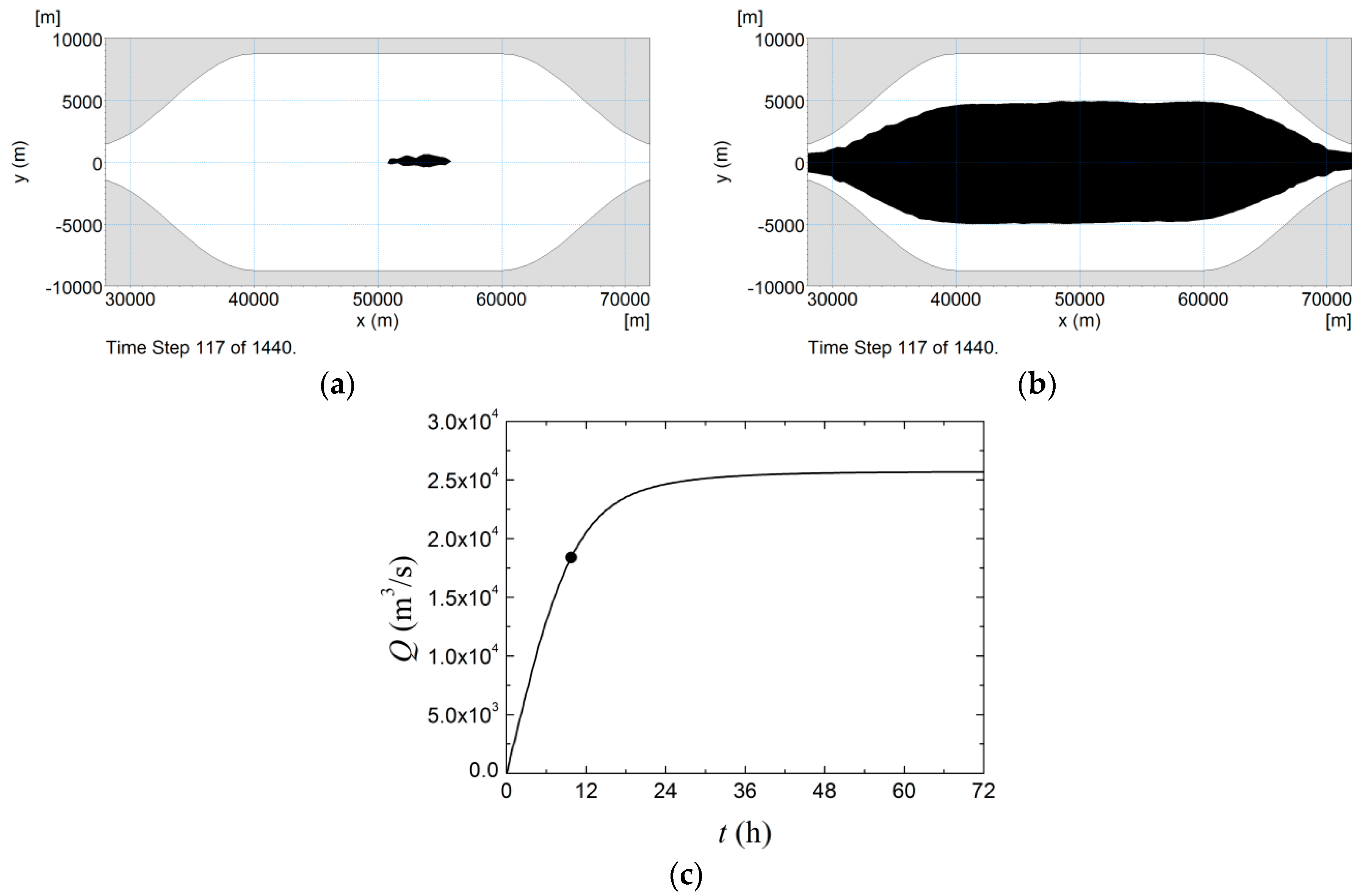
This application aims at illustrating the conclusions reached earlier regarding the return flow in flow-through gulfs. To this end, we examine the wind-induced flow in the idealized coastline and bathymetry shown in Figure 2a. It should be noted that the actual numerical domain is considerably larger than the area of the gulf shown in the figure, since it includes a wide and deep region both in the entrance of the gulf (left side) and at its exit (right side), which have (numerically) open boundaries, in order to allow the wind-induced flow to develop an accelerating inflow into the gulf, which then outflows from the other end, creating thusly a flow-through system. The dimensions of this geometry, which have been chosen to be of the same order as the natural geometry examined in the third application below, are 40 km long, 17.5 km wide and 50 m deep. The flow is created by a westerly 8 m/s wind, which exerts a surface shear stress of 0.1056 N/m². The accelerating volumetric inflow curve, produced by the numerical simulation, is shown in Figure 2c, and from this, the $\overline{A}$ parameter, given by Equation (24), can be calculated to be 0.527. Finally, λ = 1.40 and $\lambda \overline{h}$ = 46.5 m < 50 m (note that the cross-section is parabolic). As expected, the return flow (black area) first appears during the acceleration phase, at Instant 3 depicted in Figure 2a, and later becomes larger, when the flow goes into a deceleration phase. To complete the comparison with the corresponding theory, numerical simulations were repeated in the same geometry, but closing the open boundaries, rendering the numerical domain a lake. The resulting return flow, shown as the black area in Figure 2b, can be seen to be much larger than in the flow-through geometry, as expected by theory, and actually follows close enough the mean depth contour of the lake. To conclude this application, we note that exact comparison with the theoretically-predicted area of the return flow is precluded by the existence of seiches, but the predicted value falls within the numerically-simulated range.

For cases (with idealized geometries) with $\lambda \overline{h}>h_{max}$, simulations (not shown here to save space) indicate that the return flow does not appear during the acceleration phase. This means that the gulf functions as a channel, but the cross-flow profile of the longitudinal velocity is quite different from classical channel flow and is as predicted by Equation (27).

3.2. Second Application: Elongated Lake of a Parabolic Cross-Section

3.2.1. Analytical Results

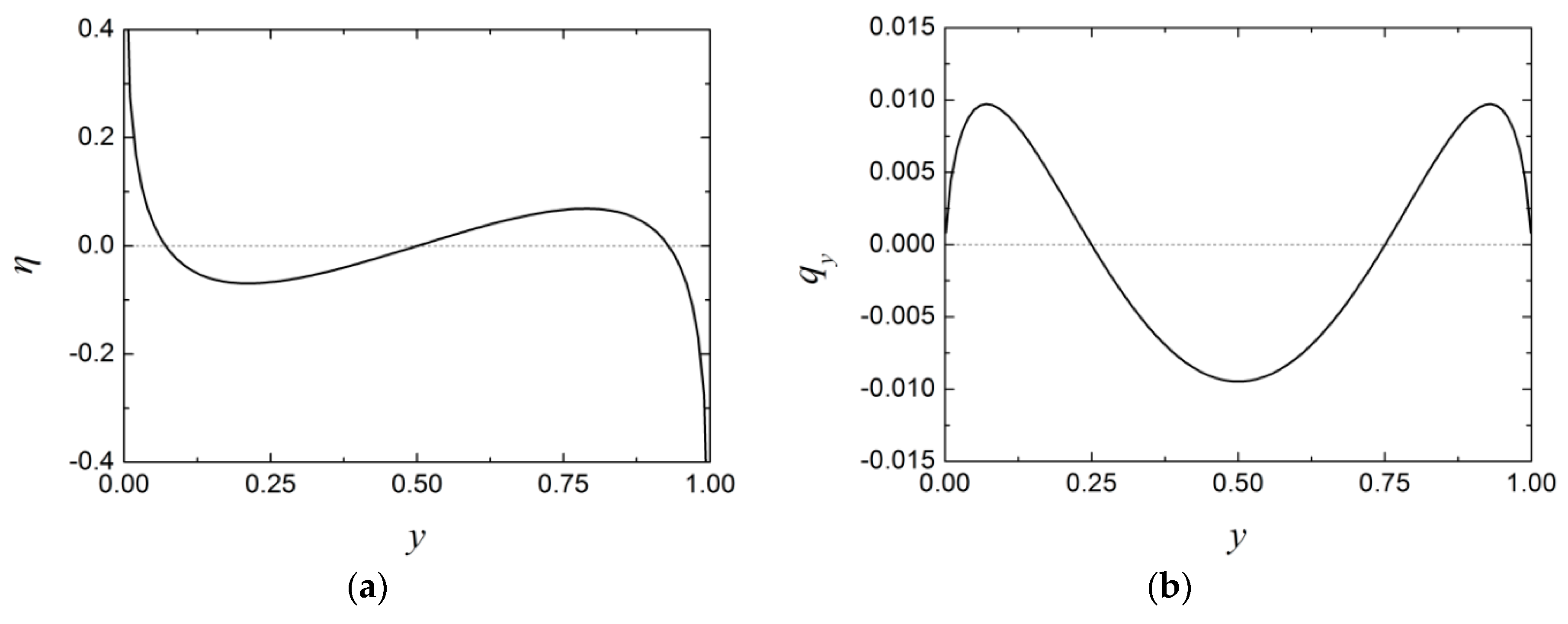
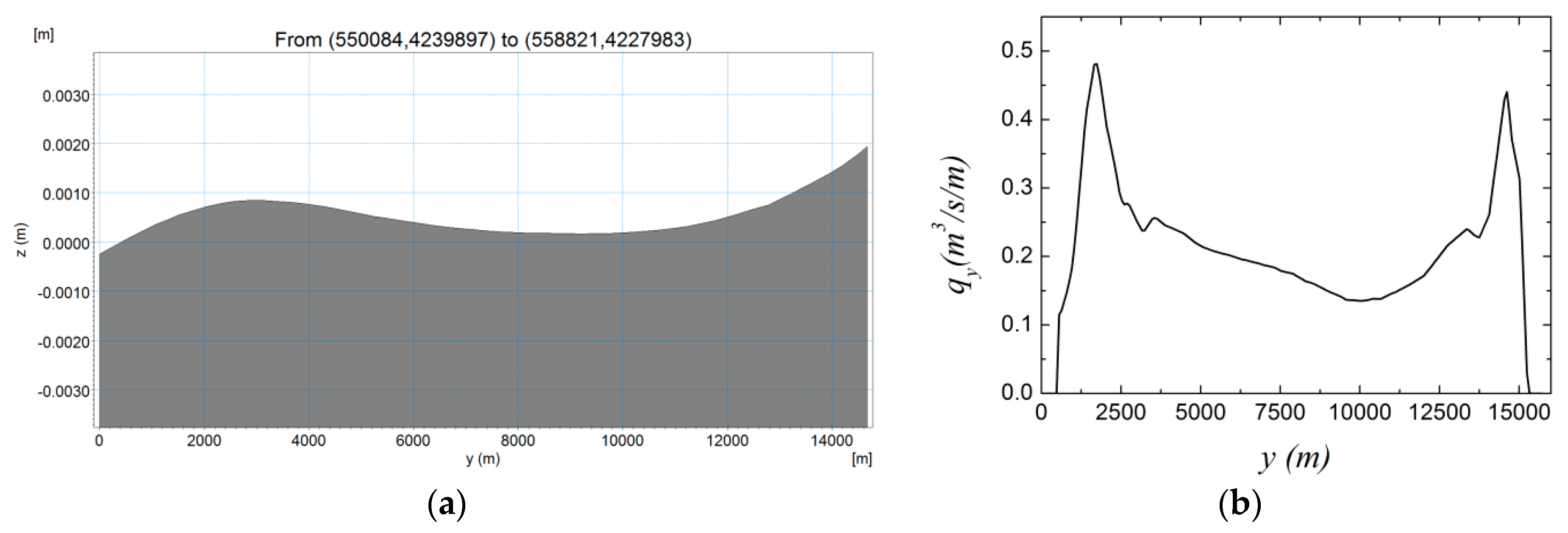
The analytically-derived Equations (34) and (36), if evaluated for a parabolic cross-section (for the details, see the Appendix A), produce the shapes given by Equations (A4) and (A5), respectively shown in Figure 3.

To give a dimensional example, for a lake having dimensions: $\mathcal{\ell }$ = 30 km, b = 4.4 km and h_max = 40 m ($\overline{h}$ = 26.7 m), a 10-m/s wind blowing for 3 h, the value of $\epsilon ,\mathcal{A},𝓀$ has been chosen so that the above theory may be used. The $q_y$ scale, given by Equation (4), is 0.4 m³/s/m, and using Figure 3, the cross-wind flux $q_y$ is of the order of 4 m³/s/m. Although this flow may seem weak, it imposes an exchange flux between littoral and pelagic regions, which may transport dissolved constituents, e.g., nutrients, thereby affecting water quality in lacustrine systems, and it is at least comparable to fluxes induced, for example, by convective cooling of lakes (e.g., [10,11]).

3.2.2. Simulation Results of Idealized Problem

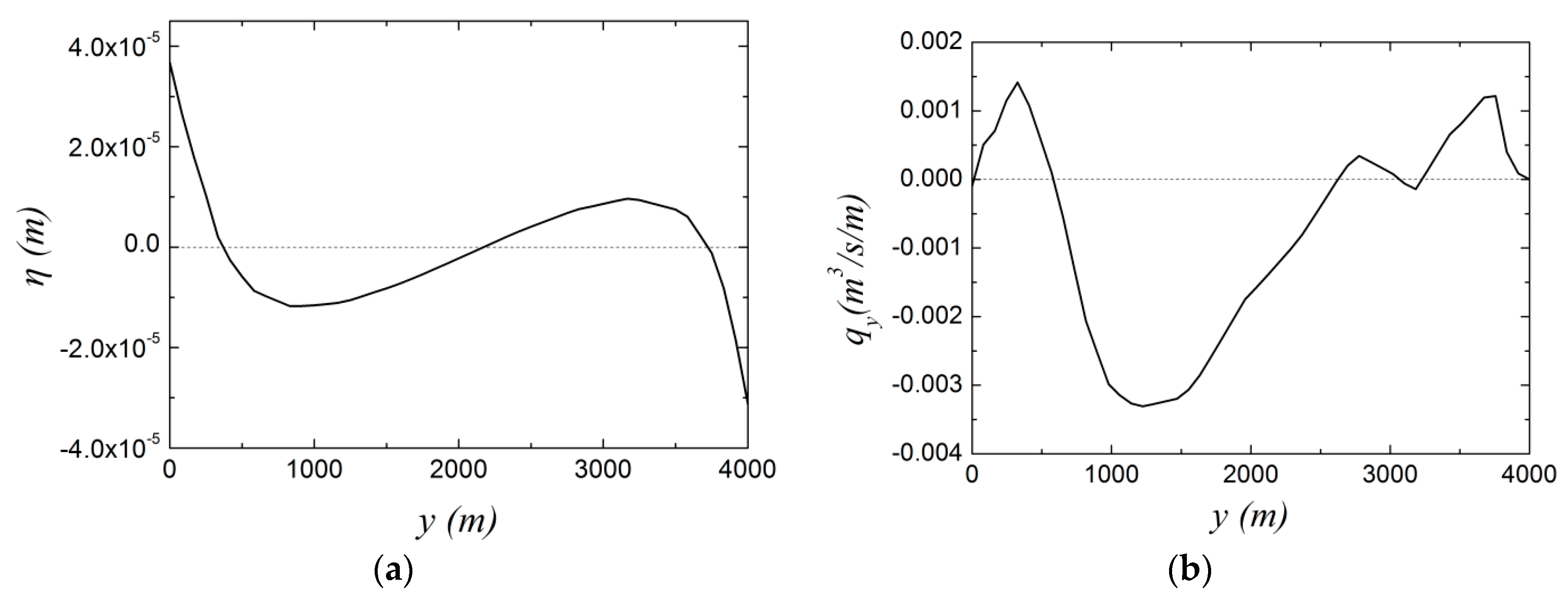
We now turn to a numerical simulation of a lake problem similar to the example discussed in the previous example. The shapes of the simulated cross-flow free-surface and the cross-flow flux that are presented in Figure 4 are to be compared with the respective shapes calculated analytically (Figure 3). It is noteworthy that, although the shape of the cross-flow free surface is excellent, the shape of the cross-flow flux is not, and the present writers have been unable to produce a more coherent $q_y$ curve, in spite of their efforts. A plausible reason for the discrepancy, besides the difficulty of simulating numerically weak second order effects, may be that the presence of seiches excites the nonlinearities of the problem, which are negligible when the seiches are absent. In spite of its non-smooth shape, the $q_y$ curve in Figure 4b presents the same basic features as the analytical $q_y$ curve in Figure 3b.

3.3. Third Application: The Gulf of Patras

The previous examples are problems defined in idealized geometries, which strictly fall within the formal requirements of the theory developed earlier. In contrast, the example to be examined in the present section is a real case application, defined in irregular geometry.

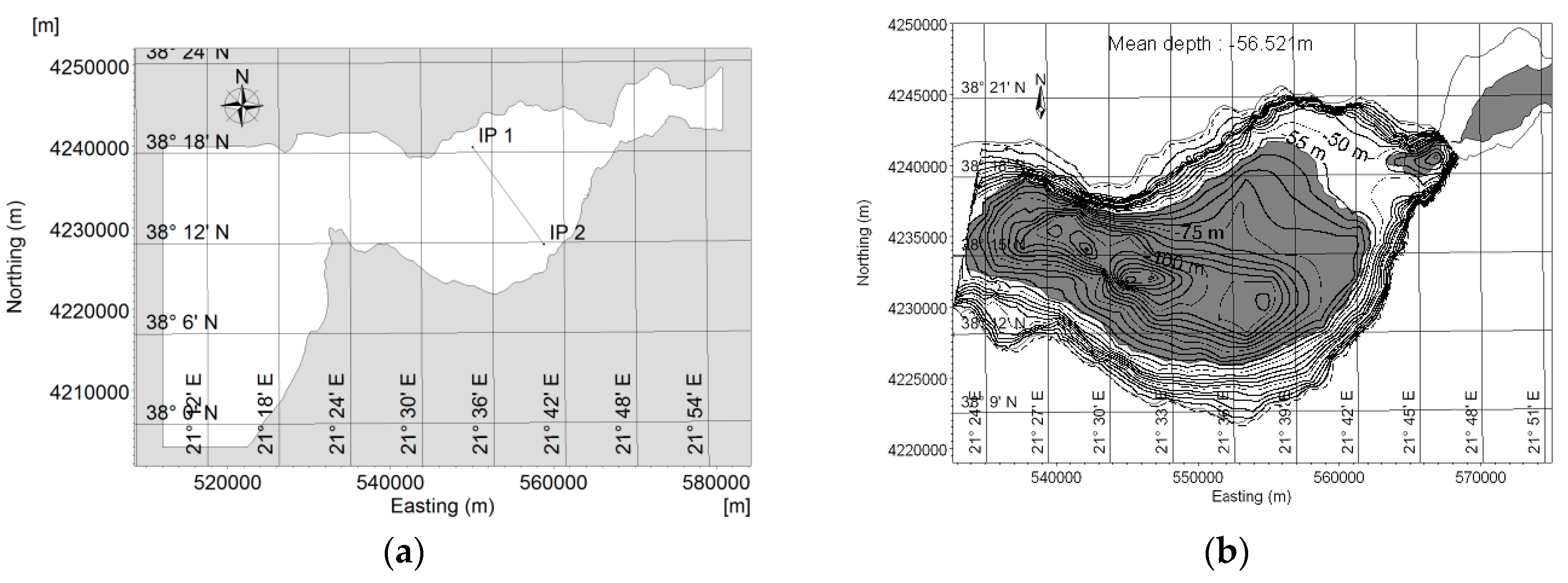
The wind-induced circulation in the Gulf of Patras, in Western Greece, has been studied using three-dimensional numerical simulations by [5]. Details of this application can be found in the original paper; here, we merely summarize pertinent details. The wider area of the Gulf, which served as the numerical domain of the simulations, is shown in Figure 5a. The Gulf proper is 40–50 km long, 10–20 km wide and 56 m in mean depth, approximately (Figure 5b).

The wind-induced circulation presents the familiar, by now, features: the S-shaped cross-flow free-surface and the M-shaped cross-flow flux, shown in Figure 6 (the fact that the M-shaped cross-flow flux does not integrate to zero is due to the presence of seiches). We believe that these features would have been difficult to interpret outside of the context of the present study. It should be noted that although Csanady’ s model and its extensions have been based on the depth integrated equations, the simulations of the present example have been three-dimensional, and this is only in order to compare the results with the present study that they have been depth integrated a posteriori.

Up to this point, we have used the numerical applications to illustrate features that have been analyzed in the above theory. At his point, we move beyond the strict bounds of the theory covering the flow acceleration, to the deceleration phase up to the steady state. This phase of the flow development has been covered by the qualitative arguments of Csanady (1973) [2], which are based, briefly, on the concept that during deceleration and at steady state, the role played in the theory by the acceleration terms is taken over by the friction terms, so that the conclusions concerning the return flow and the strong nearshore currents still hold. For the complete arguments, we refer to the original article.

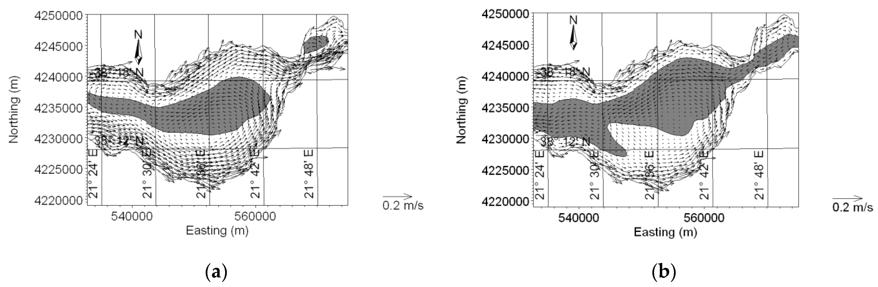
The part of the numerical domain where the local depth is larger than the mean depth is shown in Figure 5b. The steady state of the depth-averaged circulation in the Gulf induced by a 6-m/s westerly wind is shown in Figure 7, for two cases. In the panel case (Figure 7a), the Gulf functions as a flow-through gulf, i.e., as it actually is, while in the second (Figure 7b), it is artificially reduced to a lake (by numerically “closing” both of its ends). In the flow-through mode, strong nearshore currents, which had developed during the acceleration phase of the flow, can be observed to survive at steady state. The return flow is confined to the deeper region, compared to the “lake mode” of the same gulf, shown in the latter panel, which can be seen to be fairly well correlated with the deeper-than-mean-depth region in Figure 5b.

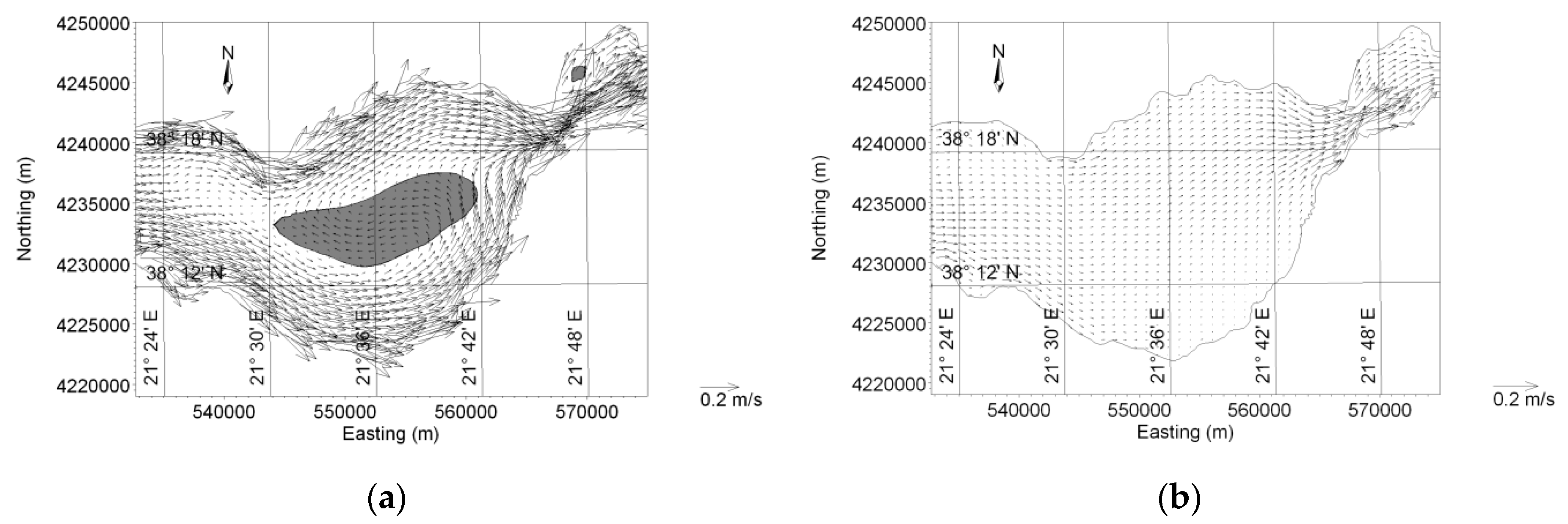
Finally, in order to demonstrate the great difference between the flow field developing under wind forcing, compared to the flow field due to the tide, we juxtapose, in Figure 8, a flow-field instant under the combined action of the wind and the tide, at quadratures (left panel) to the flow-field instant under the action of the tide alone. Again, the wind-induced circulation features are prominent, and this is so not only at quadratures, but also at the syzygies, when the tidal range is much larger (up to 40 cm) [12]. The reason is that tidal flow induces weak currents nearshore, as can be seen in Figure 8b, so that in the presence of the wind, the wind-induced currents prevail nearshore, giving rise to the same phenomenon.

3.4. Non-Uniform Cross-Flow Wind Profile

Up to this point, both in the analysis and in the applications examined, including the wind-induced flow in the Gulf of Patras, we have assumed a uniform wind field, resulting in a constant wind stress on the surface of the water body. This is clearly an idealization, especially for smaller water bodies for which the sheltering effect near the shores is evident. e.g., [13]. Detailed examination of the sheltering effect on the strong nearshore currents, examined herein, is outside the scope of the present paper. Csanady [2] has analyzed field data, which, together with numerical simulations of the time, provided the stimulus for the development of his theory. A simple modification of that theory may provide the frame for arguing that the sheltering effect should not influence decisively the creation of strong nearshore currents, as follows.

If we assume that the wind shear stress ${\tau }_x$ is a function of y, i.e., ${\tau }_x={\tau }_x\left(y\right)$, then following Csanady’s procedure, summarized in Section 2.4, we conclude that Equation (20) is modified as:

$$\frac{d\eta }{dx}=\frac{{\overline{\tau }}_x}{\rho g\overline{h}}$$

(37)

where ${\overline{\tau }}_x$ is the mean value of the surface shear stress. Therefore, Equation (21) is modified as:

$$q_x=\frac{{\overline{\tau }}_x}{\rho }t\left(\frac{{\tau }_x\left(y\right)}{{\overline{\tau }}_x}-\frac{h}{\overline{h}}\right)$$

(38)

From this equation, we conclude that if the sheltering effect is felt at up to a distance at which the depth is smaller than the mean depth, and this is a quite reasonable assumption, then no major modifications to the already reached conclusions are required. The details, however, require detailed profiles of ${\tau }_x\left(y\right)$.

4. Synopsis and Conclusions

Flow-through long gulfs share with long lakes the development, under wind forcing, of strong nearshore currents and a return flow, in the depth-integrated sense, at the deeper regions. The difference is that while the return, upwind flow develops in lakes in regions deeper than the mean depth $\overline{h}$, in flow-through gulfs, it develops in regions deeper than the corrected mean depth, $\lambda \overline{h}$, where the parameter $\lambda$, given by Equation (28), can be calculated given the gulf’s cross-section, the wind shear stress and the volumetric inflow into the gulf. When the corrected mean depth is deeper than the gulf’s maximum depth, the return flow forms when the flow decelerates on its way to reaching the steady state.

Characteristic flow features in the lake flow, shared by flow-through gulfs, are the cross-flow shape of the free surface and the cross-flow shorewise flux, which will form under the influence of the Coriolis force, in short enough times. These features may appear in numerical simulations of complex real-life applications, even in cases that marginally satisfy the requirements of the theory, and when identified, they help interpret the results of the numerical simulations. The shorewise flux, even though it is weak, may be of importance in environmental applications.

References

- Liggett, J.A.; Hadjitheodorou, C. Circulation in shallow homogeneous lakes. J. Hydraul. Div. 1969, 95, 609–620. [Google Scholar]
- Csanady, G.T. Wind-Induced Barotropic Motions in Long Lakes. J. Phys. Oceanogr. 1973, 3, 429–438. [Google Scholar] [CrossRef]
- Cioffi, F.; Gallerano, F.; Napoli, E. Three-dimensional numerical simulation of wind-driven flows in closed channels and basins. J. Hydraul. Res. 2005, 43, 290–301. [Google Scholar] [CrossRef]
- Borthwick, A.G.L.; Cruz León, S.; Józsa, J. Adaptive quadtree model of shallow-flow hydrodynamics. J. Hydraul. Res. 2000, 39, 413–424. [Google Scholar] [CrossRef]
- Fourniotis, N.T.; Horsch, G.M. Three-dimensional numerical simulation of, wind-induced barotropic circulation in the Gulf of Patras. Ocean Eng. 2010, 37, 355–364. [Google Scholar] [CrossRef]
- Dean, R.G.; Dalrymple, R.A. Water Wave Mechanics for Engineers and Scientists; World Scientific Publishing Company: Singapore, 1991; p. 368. [Google Scholar]
- Lamb, K.G. Course Notes for AMATH 732; Department of Applied Mathematics, University of Waterloo: Waterloo, ON, Canada, 2010. [Google Scholar]
- Danish Hydraulic Institute (DHI). MIKE 21 FLOW MODEL FM, Hydrodynamic Module—User Guide; DHI Horsholm: Hørsholm, Denmark, 2005; p. 132. [Google Scholar]
- Danish Hydraulic Institute (DHI). MIKE 3 FLOW MODEL FM, Hydrodynamic Module—User Guide; DHI Horsholm: Hørsholm, Denmark, 2007; p. 138. [Google Scholar]
- Stefan, H.G.; Horsch, G.M.; Barko, J.W. A model for the estimation of convective exchange in the littoral region of a shallow lake during cooling. Hydrobiologia 1989, 174, 225–234. [Google Scholar] [CrossRef]
- Horsch, G.M.; Stefan, H.G. Convective circulation in littoral water due to surface cooling. Limnol. Oceanogr. 1988, 33, 1068–1083. [Google Scholar] [CrossRef]
- Horsch, G.M.; Fourniotis, N.T. Wintertime Tidal Hydrodynamics in the Gulf of Patras, Greece. J. Coast. Res. 2017, 33, 1305–1314. [Google Scholar] [CrossRef]
- Markfort, C.D.; Perez, A.L.S.; Thill, J.W.; Jaster, D.A.; Porté-Agel, F.; Stefan, H.G. Wind sheltering of a lake by a tree canopy or bluff topography. Water Resour. Res. 2010, 46, 1–13. [Google Scholar] [CrossRef]
Figure 1.
Schematic diagram of a long, flow-through, semi-enclosed gulf with a regular trunk section, in which depth contours are nearly parallel.
Figure 2.
Wind-induced flow in: (a) a flow-through gulf; (b) a lake-like water body of the same bathymetry. The white region denotes flow in the direction of the wind and the black opposite to the wind. (c) Volumetric inflow into the gulf as a function of time. The dot denotes the time during the flow acceleration at which the return flow, depicted in (a), first appears.
Figure 3.
The O(ε,0,0) shapes of the dimensionless (a) cross-flow free-surface and (b) cross-flow flux.
Figure 4.
(a) The cross-flow free-surface and (b) the cross-flow flux, in the trunk region for numerically-simulated flow in idealized geometry.
Figure 5.
(a) The numerical domain for the simulations of the wind-induced circulation in the Gulf of Patras. The profiles studied below have been taken along the line IP1-IP2; (b) the Gulf of Patras proper. The dark region is deeper than the mean depth.
Figure 6.
(a) The cross-flow free-surface and (b) the cross-flow flux, along the line IP1-IP2 (Figure 5) in the Gulf of Patras, for numerically-simulated flow, induced by a 6-m/s westerly wind.
Figure 7.
Steady state flow in the Gulf of Patras induced by a 6 m/s westerly wind. (a) In flow-through mode (b) in “lake” mode.
Figure 8.
(a) Combined wind and tidal flow and (b) purely tidal flow, both in quadratures in the Gulf of Patras.
© 2018 by the authors. Licensee MDPI, Basel, Switzerland. This article is an open access article distributed under the terms and conditions of the Creative Commons Attribution (CC BY) license (http://creativecommons.org/licenses/by/4.0/).
Share and Cite
MDPI and ACS Style
Horsch, G.M.; Fourniotis, N.T. On Strong Nearshore Wind-Induced Currents in Flow-Through Gulfs: Variations on a Theme by Csanady. Water 2018, 10, 652. https://doi.org/10.3390/w10050652
AMA Style
Horsch GM, Fourniotis NT. On Strong Nearshore Wind-Induced Currents in Flow-Through Gulfs: Variations on a Theme by Csanady. Water. 2018; 10(5):652. https://doi.org/10.3390/w10050652
Chicago/Turabian StyleHorsch, Georgios M., and Nikolaos Th. Fourniotis. 2018. "On Strong Nearshore Wind-Induced Currents in Flow-Through Gulfs: Variations on a Theme by Csanady" Water 10, no. 5: 652. https://doi.org/10.3390/w10050652
Note that from the first issue of 2016, this journal uses article numbers instead of page numbers. See further details here.