Simulation of Crop Growth and Water-Saving Irrigation Scenarios for Lettuce: A Monsoon-Climate Case Study in Kampong Chhnang, Cambodia


Abstract
:1. Introduction
2. Materials and Methods
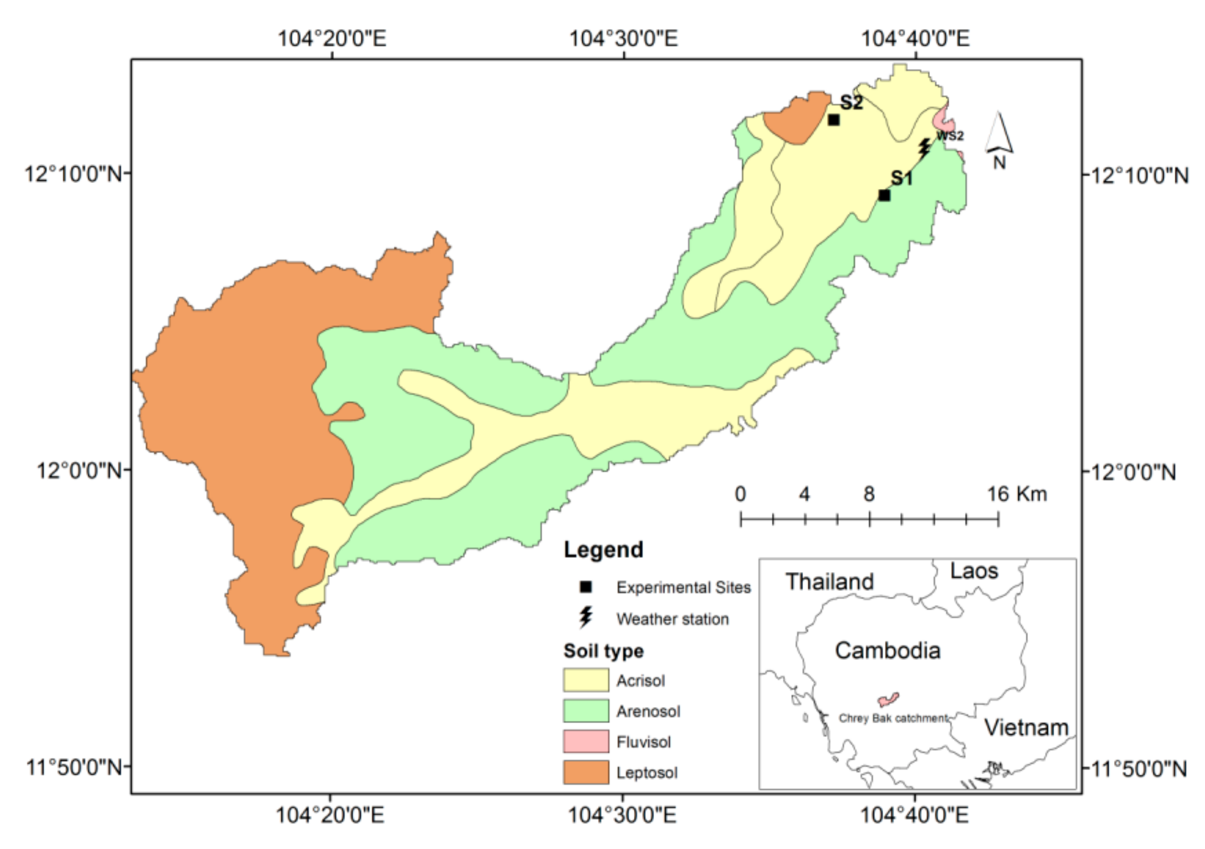
2.1. Experimental Sites
2.2. Data Collection and Measurement
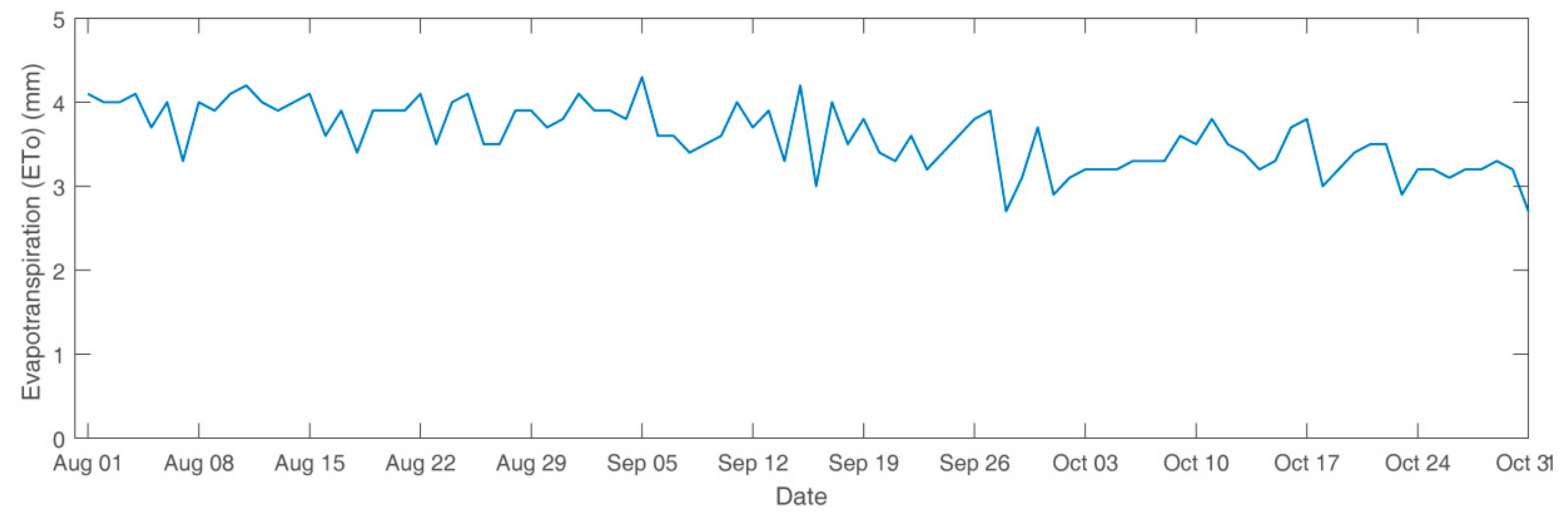
2.2.1. Climate Data
2.2.2. Soil Data
2.2.3. Crop Data
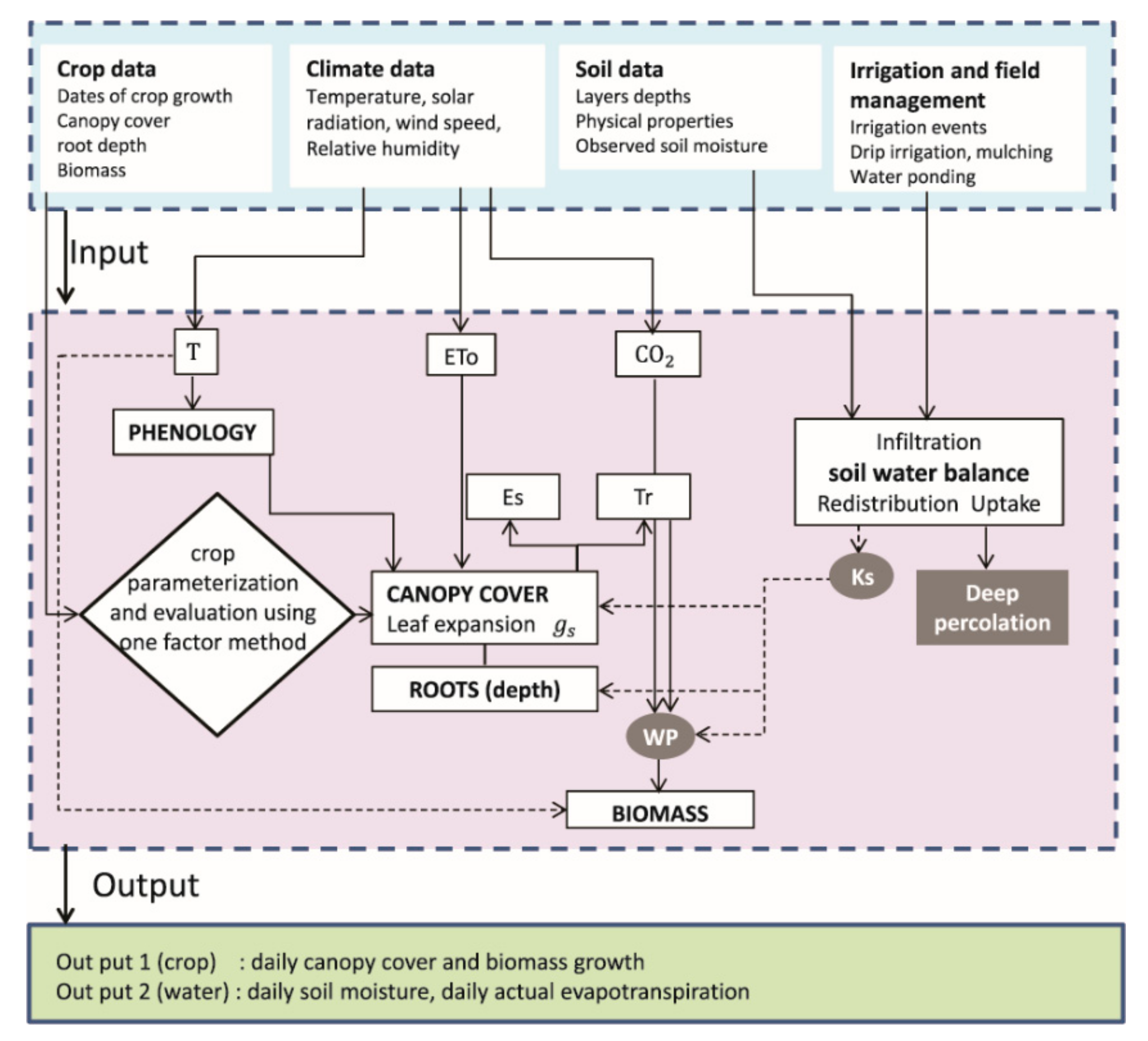
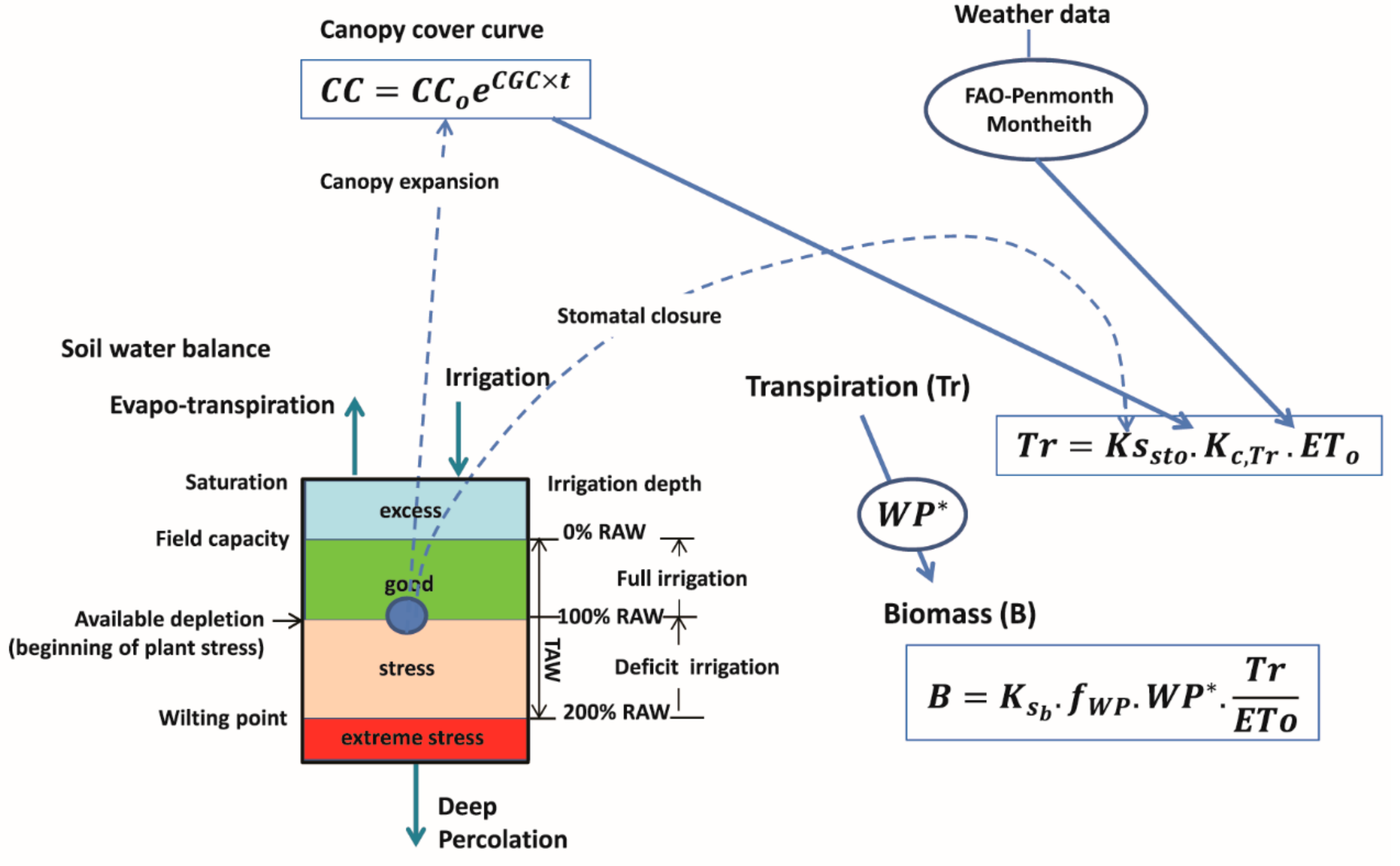
2.3. AquaCrop Model
2.4. Model Parameterisation
2.5. Irrigation Scenarios
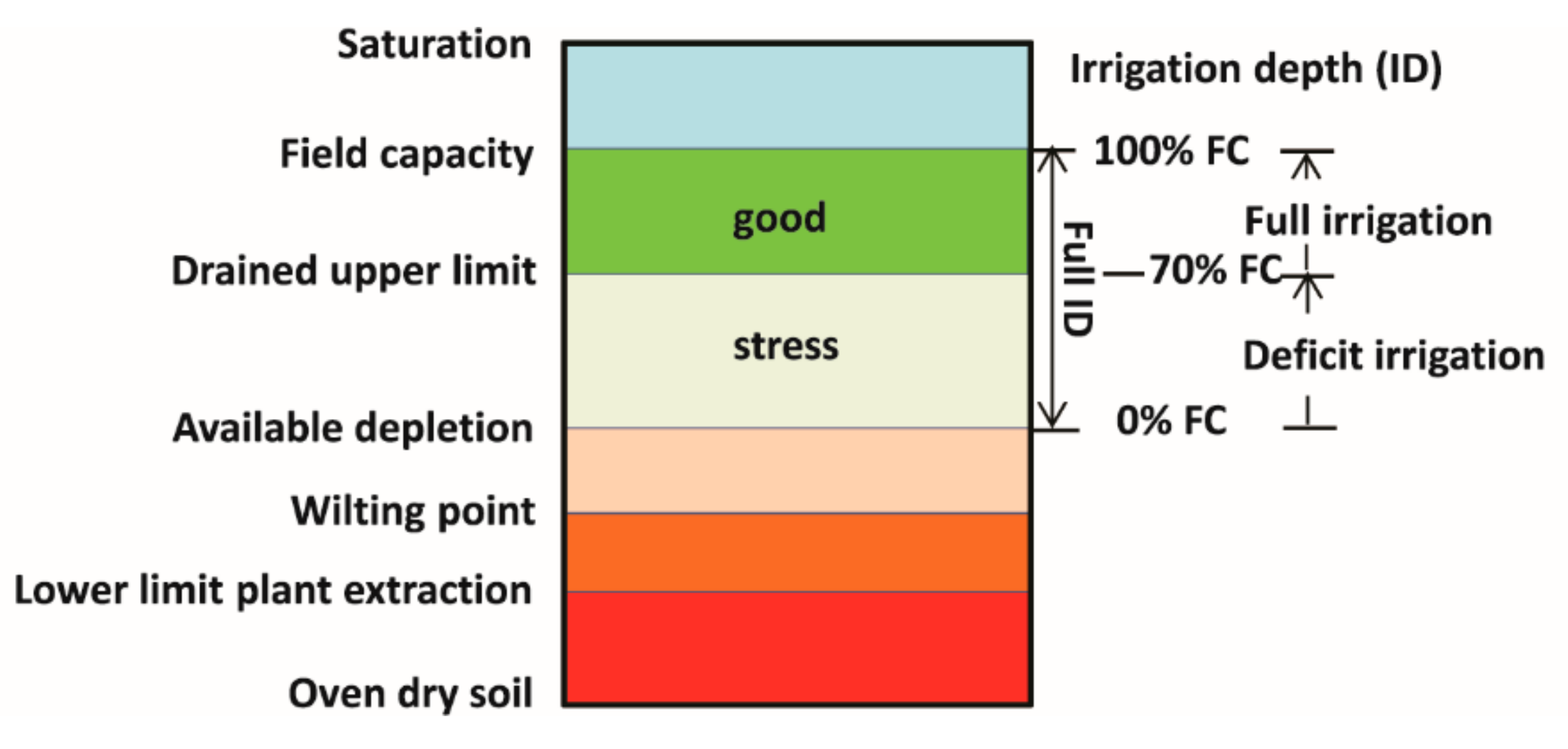
2.5.1. Varied RAW Threshold Irrigation Scenarios
- Soil water content depleted until a fixed lower threshold (RAW) and refill to field capacity (time criteria).
- Irrigation dose can be determined by the following Equation (8) [87].where ID is irrigation depth (mm), , p is soil water depletion threshold, set to 0.3 for lettuce recommended by [69], and is root depth (m). TAW is the amount of water that a crop can extract from its root zone [88]. is field capacity, that is, the amount of water well-drained soil should hold against gravitational forces (m3 m−3) [88]. PWP is permanent wilting point, referring to soil water content when a plant fails to recover its turgidity on watering (m3 m−3) [88]. RAW is readily available soil water, referring to the fraction of TAW that a crop can extract from the root zone without suffering water stress [88]. AD is allowable depletion, defined as the percentage of RAW that can be depleted before irrigation water has to be applied.
2.5.2. Varied Field Capacity Threshold Irrigation Scenarios
3. Results
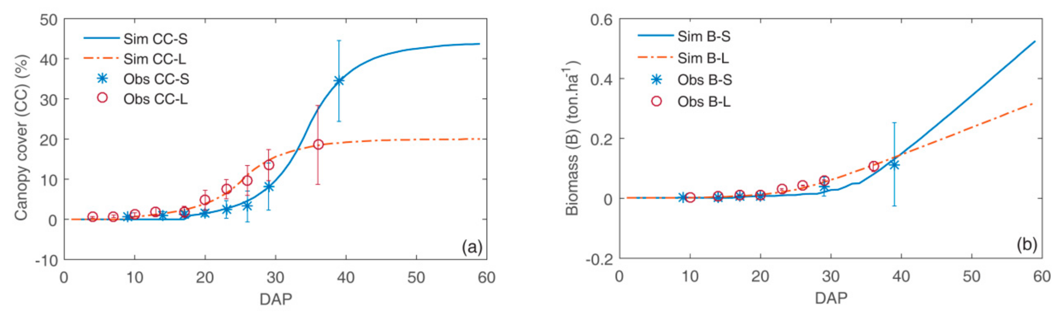
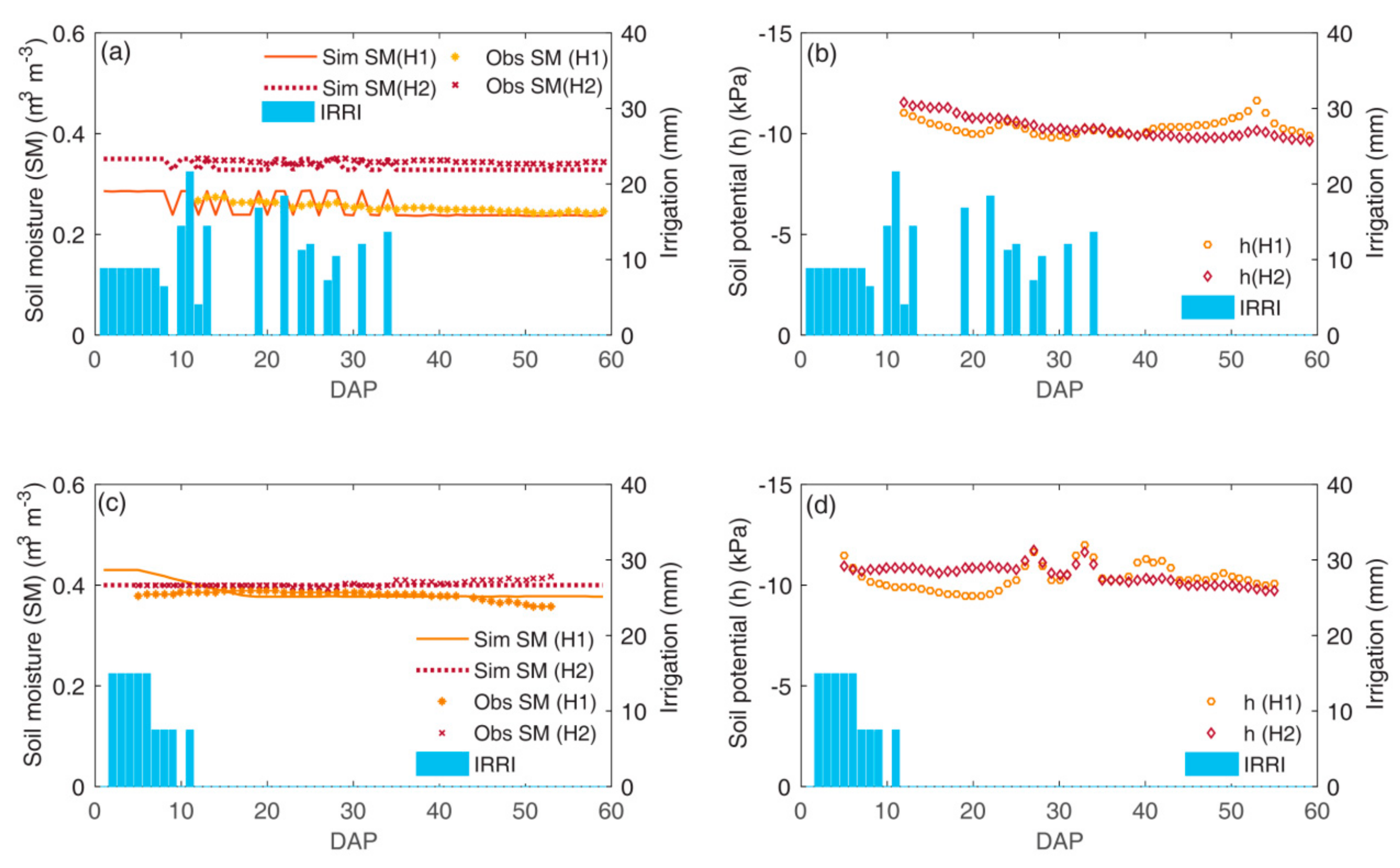
3.1. Plant Growth and Soil Moisture Status
3.2. Model Parameterisation and Evaluation
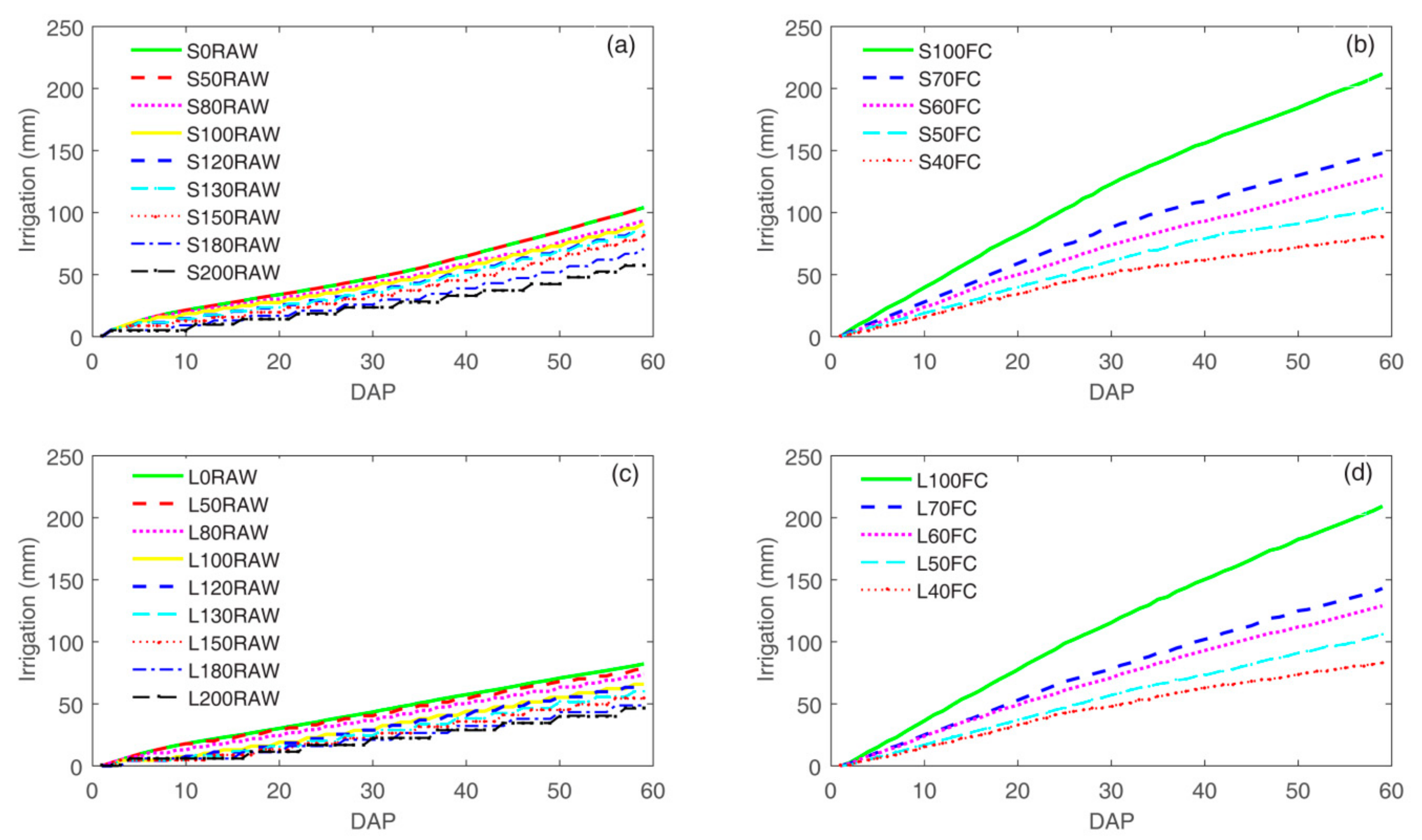
3.3. Irrigation Scenarios
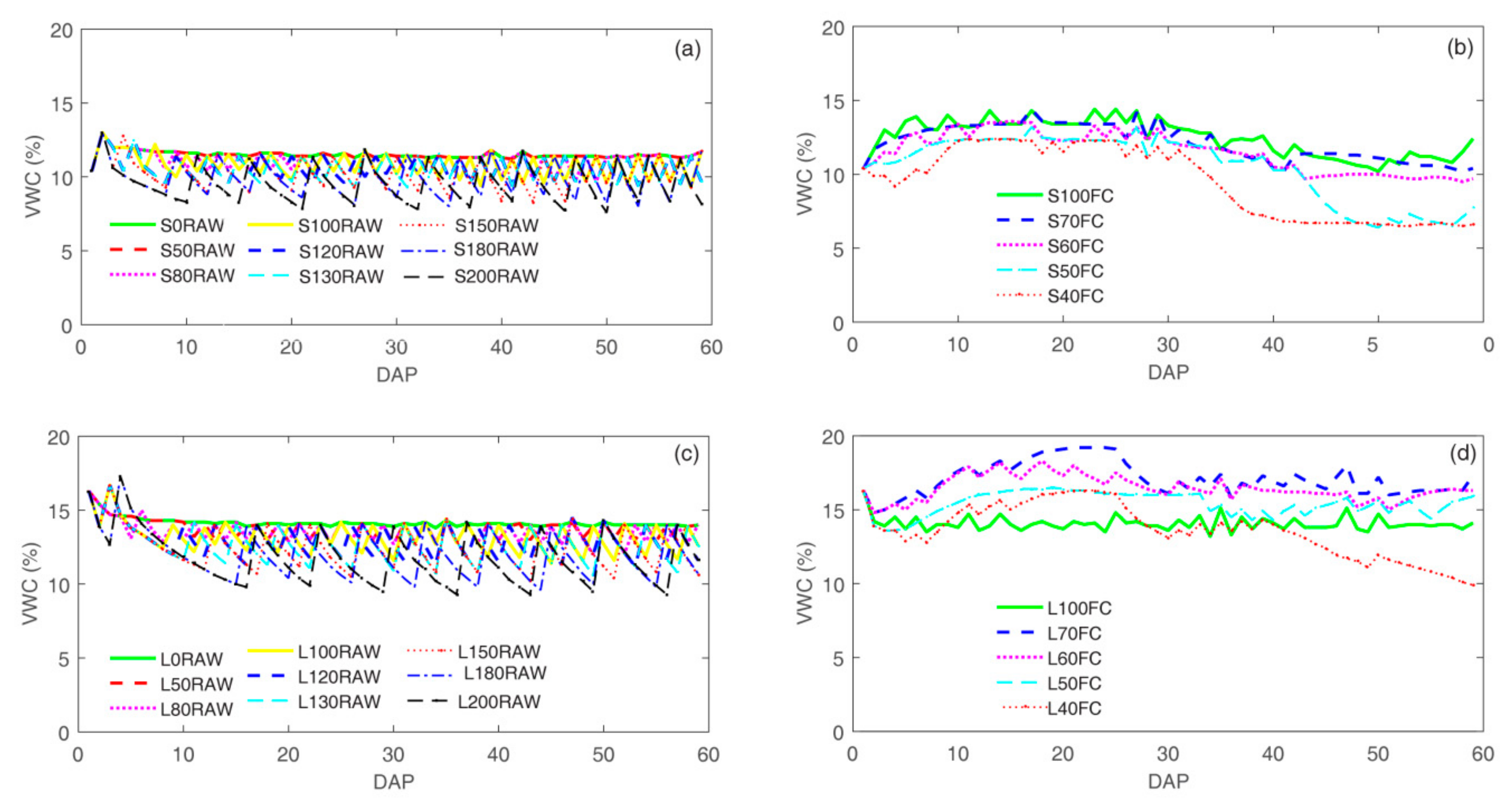
3.3.1. Irrigation and Soil Moisture Response
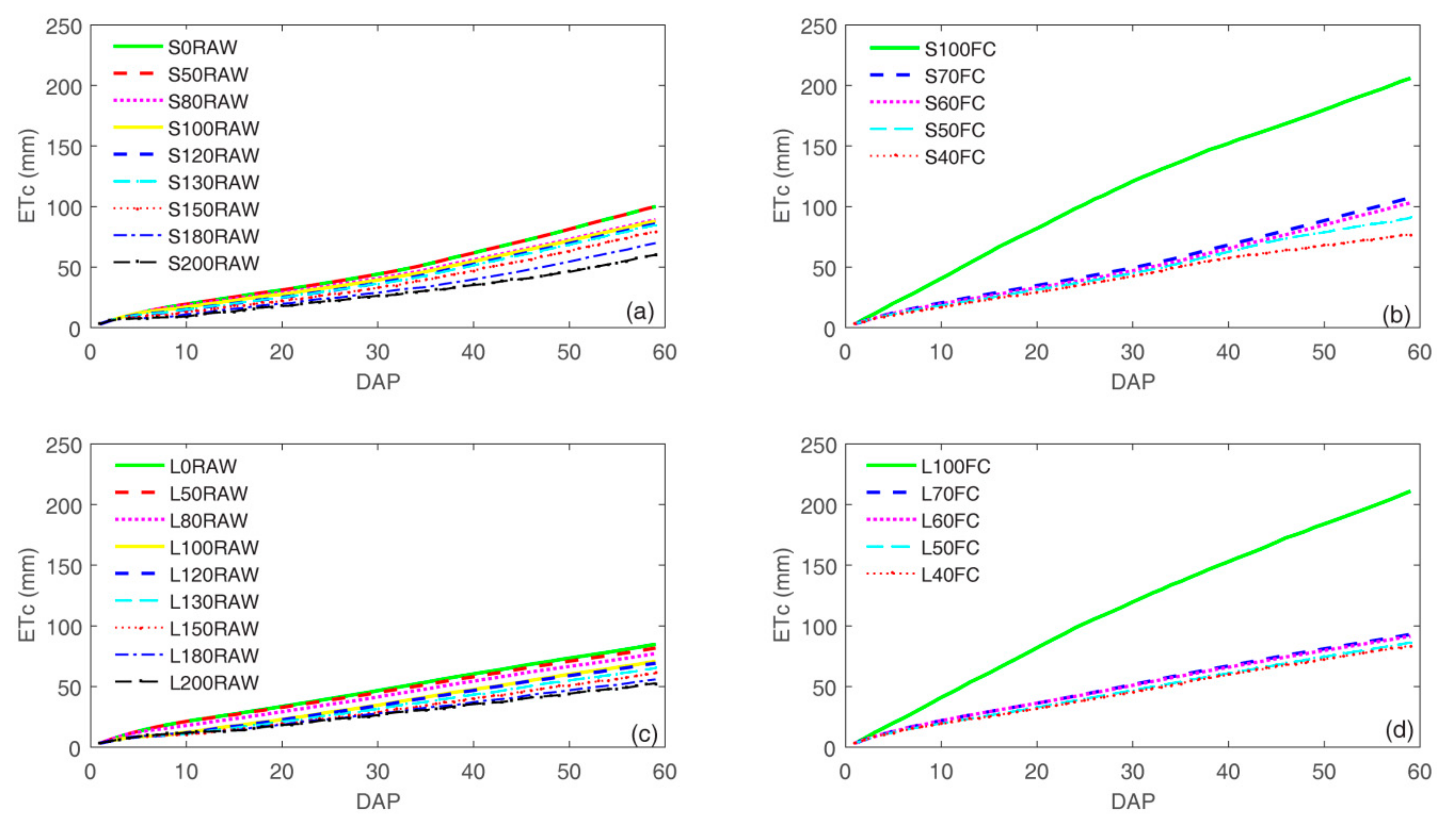
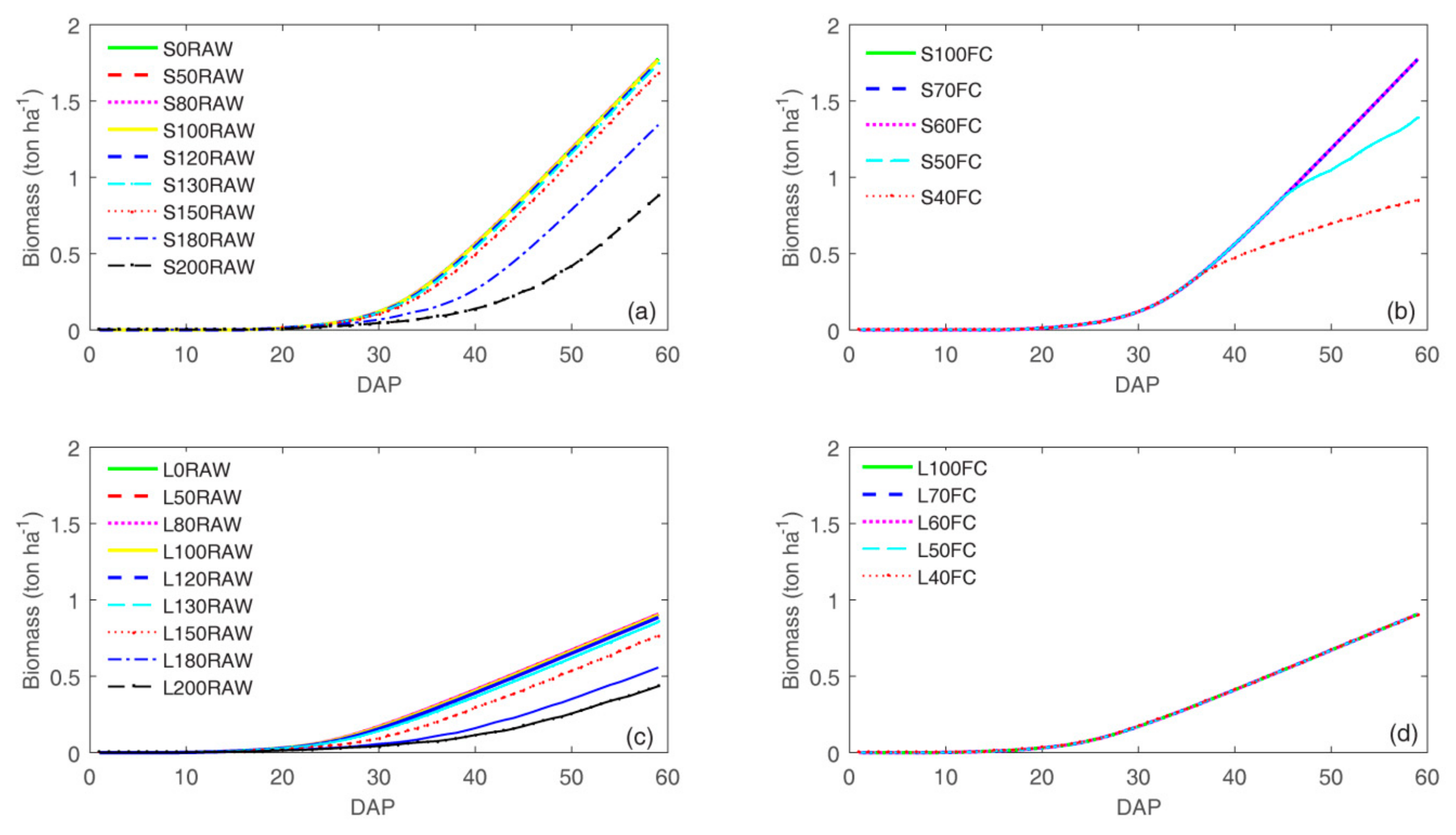
3.3.2. Crop Evapotranspiration and Biomass Growth Response
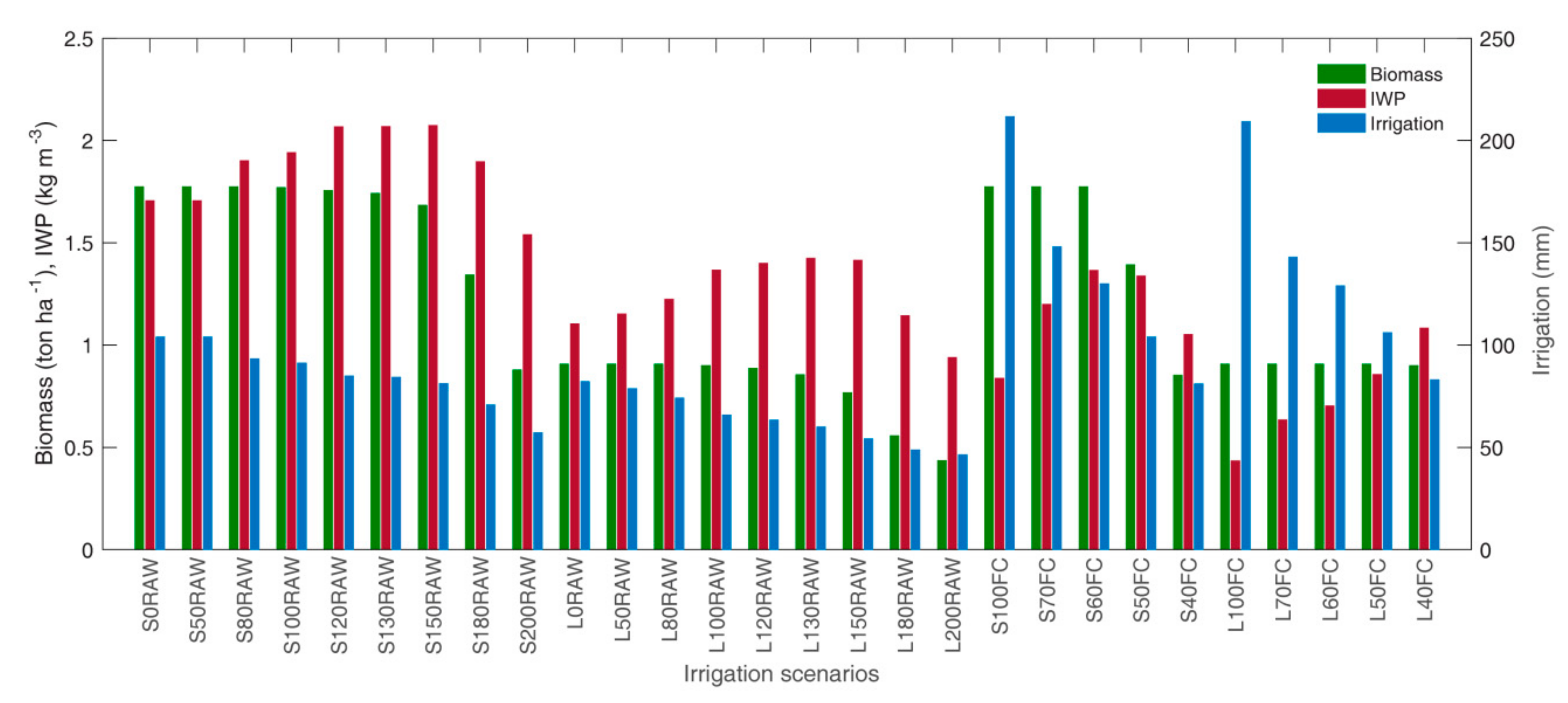
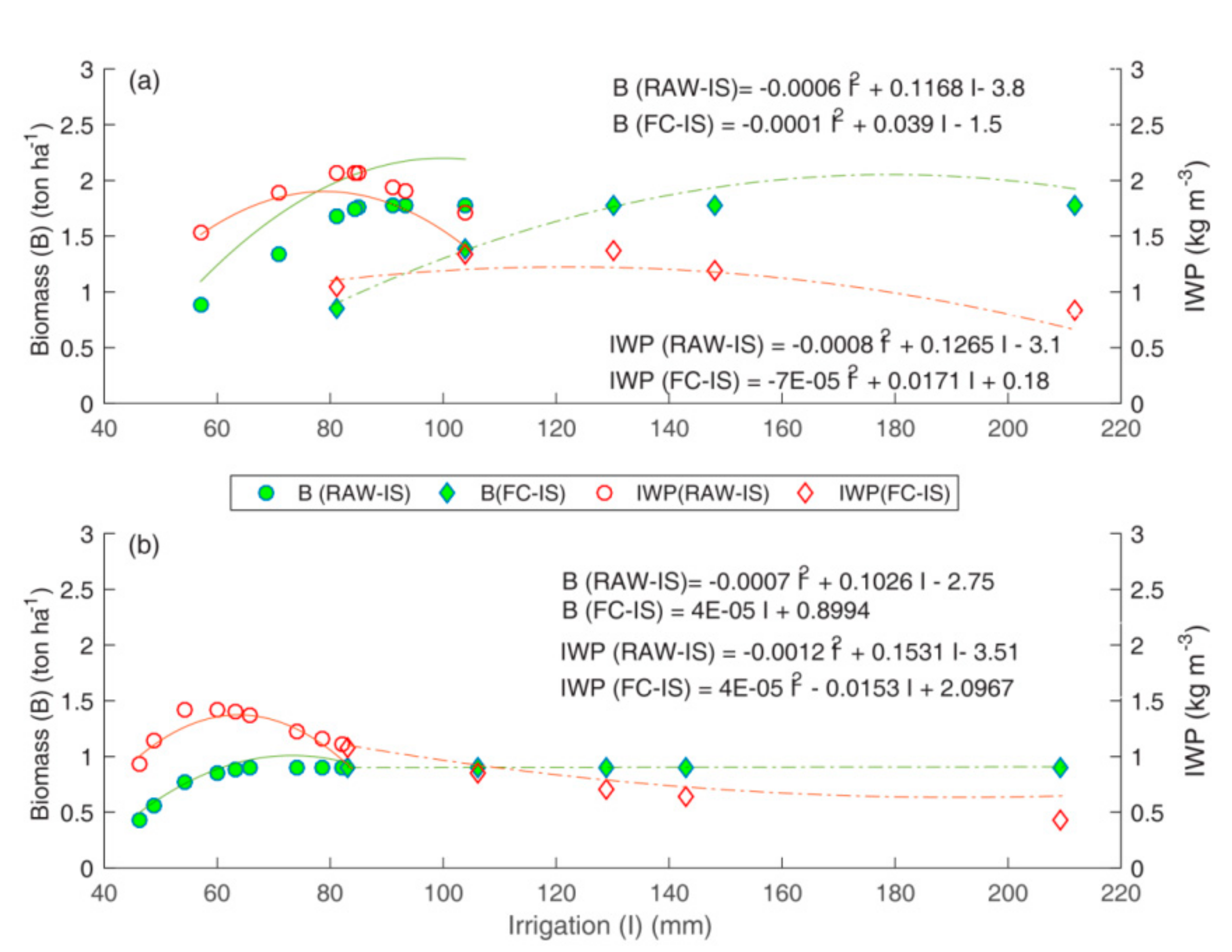
3.3.3. Relationship between Water Productivity and Irrigation Scenarios
3.3.4. Limitation
4. Conclusions
Author Contributions
Acknowledgments
Conflicts of Interest
References
- Hoekstra, A.Y.; Wiedmann, T.O. Humanity’s Unsustainable Environmental Footprint. Science 2014, 344, 1114–1117. [Google Scholar] [CrossRef] [PubMed]
- Bae, J.; Dall’erba, S. Crop Production, Export of Virtual Water and Water-Saving Strategies in Arizona. Ecol. Econ. 2018, 146, 148–156. [Google Scholar] [CrossRef]
- Rodríguez-Ferrero, N.; Salas-Velasco, M.; Sanchez-Martínez, M.T. Assessment of Productive Efficiency in Irrigated Areas of Andalusia. Int. J. Water Resour. Dev. 2010, 26, 365–379. [Google Scholar] [CrossRef]
- Chartres, C. Is Water Scarcity a Constraint to Feeding Asia’s Growing Population? Int. J. Water Resour. Dev. 2014, 30, 28–36. [Google Scholar] [CrossRef]
- Jaramillo, F.; Destouni, G. Local Flow Regulation and Irrigation Raise Global Human Water Consumption and Footprint. Science 2015, 350, 1248–1251. [Google Scholar] [CrossRef] [PubMed]
- Toumi, J.; Er-Raki, S.; Ezzahar, J.; Khabba, S.; Jarlan, L.; Chehbouni, A. Performance Assessment of AquaCrop Model for Estimating Evapotranspiration, Soil Water Content and Grain Yield of Winter Wheat in Tensift Al Haouz (Morocco): Application to Irrigation Management. Agric. Water Manag. 2016, 163, 219–235. [Google Scholar] [CrossRef]
- Linker, R.; Ioslovich, I. Assimilation of Canopy Cover and Biomass Measurements in the Crop Model AquaCrop. Biosyst. Eng. 2017, 162, 57–66. [Google Scholar] [CrossRef]
- Touch, V.; Martin, R.J.; Scott, J.F.; Cowie, A.; Liu, D.L. Climate Change Adaptation Options in Rainfed Upland Cropping Systems in the Wet Tropics: A Case Study of Smallholder Farms in North-West Cambodia. J. Environ. Manag. 2016, 182, 238–246. [Google Scholar] [CrossRef] [PubMed]
- Chhinh, N.; Millington, A. Drought Monitoring for Rice Production in Cambodia. Climate 2015, 3, 792–811. [Google Scholar] [CrossRef]
- Montgomery, S.C.; Martin, R.J.; Guppy, C.; Wright, G.C.; Tighe, M.K. Farmer Knowledge and Perception of Production Constraints in Northwest Cambodia. J. Rural Stud. 2017, 56, 12–20. [Google Scholar] [CrossRef]
- Moreira, M.A.; Dos Santos, C.A.P.; Lucas, A.A.T.; Bianchini, F.G.; De Souza, I.M.; Viégas, P.R.A. Lettuce Production according to Different Sources of Organic Matter and Soil Cover. Agric. Sci. 2014, 5, 99–105. [Google Scholar] [CrossRef]
- Valenzuela, H.R.; Bernard, K.; John, C. Lettuce Production Guidelines for Hawaii; University of Hawaii: Honolulu, HI, USA, 1996. [Google Scholar]
- Cahn, M.; Johnson, L. New Approaches to Irrigation Scheduling of Vegetables. Horticulturae 2017, 3, 1–20. [Google Scholar] [CrossRef]
- Domingues, D.S.; Takahashi, H.W.; Camara, C.A.P.; Nixdorf, S.L. Automated System Developed to Control pH and Concentration of Nutrient Solution Evaluated in Hydroponic Lettuce Production. Comput. Electron. Agric. 2012, 84, 53–61. [Google Scholar] [CrossRef]
- Sokhen, C.; Kanika, D.; Moustier, P. Vegetable Market Flows and Chains in Phnom Penh; CIRAD-AVRDC-French MOFA: Hanoi, Vietnam, 2004. [Google Scholar]
- De Bon, H.; Parrot, L.; Moustier, P. Sustainable Urban Agriculture in Developing Countries. A Review. Agron. Sustain. Dev. 2010, 30, 21–32. [Google Scholar] [CrossRef]
- Morris, S.; Davies, W.; Baines, R.N. Challenges and Opportunities for Increasing Competitiveness of Vegetable Production in Cambodia. Acta Hortic. 2013, 1006, 253–260. [Google Scholar] [CrossRef]
- Xue, J.; Huo, Z.; Wang, F.; Kang, S.; Huang, G. Untangling the Effects of Shallow Groundwater and Deficit Irrigation on Irrigation Water Productivity in Arid Region: New Conceptual Model. Sci. Total Environ. 2018, 619–620, 1170–1182. [Google Scholar] [CrossRef] [PubMed]
- Adu, M.O.; Yawson, D.O.; Armah, F.A.; Asare, P.A.; Frimpong, K.A. Meta-Analysis of Crop Yields of Full, Deficit, and Partial Root-Zone Drying Irrigation. Agric. Water Manag. 2018, 197, 79–90. [Google Scholar] [CrossRef]
- Liu, Y.; Luo, Y. A Consolidated Evaluation of the FAO-56 Dual Crop Coefficient Approach Using the Lysimeter Data in the North China Plain. Agric. Water Manag. 2010, 97, 31–40. [Google Scholar] [CrossRef]
- Verstraeten, W.W.; Veroustraete, F.; Feyen, J. Assessment of Evapotranspiration and Soil Moisture Content across Different Scales of Observation. Sensors 2008, 8, 70–117. [Google Scholar] [CrossRef] [PubMed]
- Hunsaker, D.J.; French, A.N.; Waller, P.M.; Bautista, E.; Thorp, K.R.; Bronson, K.F.; Andrade-Sanchez, P. Comparison of Traditional and ET-Based Irrigation Scheduling of Surface-Irrigated Cotton in the Arid Southwestern USA. Agric. Water Manag. 2015, 159, 209–224. [Google Scholar] [CrossRef]
- Thompson, R.B.; Gallardo, M.; Valdez, L.C.; Fernández, M.D. Determination of Lower Limits for Irrigation Management Using in Situ Assessments of Apparent Crop Water Uptake Made with Volumetric Soil Water Content Sensors. Agric. Water Manag. 2007, 92, 13–28. [Google Scholar] [CrossRef]
- Ferreira, M.I.; Conceição, N.; Malheiro, A.C.; Silvestre, J.M.; Silva, R.M. Water Stress Indicators and Stress Functions to Calculate Soil Water Depletion in Deficit Irrigated Grapevine and Kiwi. Acta Hortic. 2017, 1150, 119–126. [Google Scholar] [CrossRef]
- Li, S.; Kang, S.; Li, F.; Zhang, L. Evapotranspiration and Crop Coefficient of Spring Maize with Plastic Mulch Using Eddy Covariance in Northwest China. Agric. Water Manag. 2008, 95, 1214–1222. [Google Scholar] [CrossRef]
- Kashyap, P.S.; Panda, R.K. Evaluation of Evapotranspiration Estimation Methods and Development of Crop-Coefficients for Potato Crop in a Sub-Humid Region. Agric. Water Manag. 2001, 50, 9–25. [Google Scholar] [CrossRef]
- Inthavong, T.; Tsubo, M.; Fukai, S. A Water Balance Model for Characterization of Length of Growing Period and Water Stress Development for Rainfed Lowland Rice. Field Crop. Res. 2011, 121, 291–301. [Google Scholar] [CrossRef]
- Davis, S.L.; Dukes, M.D. Irrigation Scheduling Performance by Evapotranspiration-Based Controllers. Agric. Water Manag. 2010, 98, 19–28. [Google Scholar] [CrossRef]
- Kukal, S.S.; Hira, G.S.; Sidhu, A.S. Soil Matric Potential-Based Irrigation Scheduling to Rice (Oryza sativa). Irrig. Sci. 2005, 23, 153–159. [Google Scholar] [CrossRef]
- Pereira, L.S.; Paredes, P.; Sholpankulov, E.D.; Inchenkova, O.P.; Teodoro, P.R.; Horst, M.G. Irrigation Scheduling Strategies for Cotton to Cope with Water Scarcity in the Fergana Valley, Central Asia. Agric. Water Manag. 2009, 96, 723–735. [Google Scholar] [CrossRef]
- Pereira, L.S.; Cordery, I.; Iacovides, I. Improved Indicators of Water Use Performance and Productivity for Sustainable Water Conservation and Saving. Agric. Water Manag. 2012, 108, 39–51. [Google Scholar] [CrossRef]
- Afzal, M.; Battilani, A.; Solimando, D.; Ragab, R. Improving Water Resources Management Using Different Irrigation Strategies and Water Qualities: Field and Modelling Study. Agric. Water Manag. 2016, 176, 40–54. [Google Scholar] [CrossRef]
- Geerts, S.; Raes, D. Deficit Irrigation as an on-Farm Strategy to Maximize Crop Water Productivity in Dry Areas. Agric. Water Manag. 2009, 96, 1275–1284. [Google Scholar] [CrossRef] [Green Version]
- Chai, Q.; Gan, Y.; Zhao, C.; Xu, H.L.; Waskom, R.M.; Niu, Y.; Siddique, K.H.M. Regulated Deficit Irrigation for Crop Production under Drought Stress. A Review. Agron. Sustain. Dev. 2016, 36, 1–21. [Google Scholar] [CrossRef]
- Lopez, J.R.; Winter, J.M.; Elliott, J.; Ruane, A.C.; Porter, C.; Hoogenboom, G. Integrating Growth Stage Deficit Irrigation into a Process Based Crop Model. Agric. For. Meteorol. 2017, 243, 84–92. [Google Scholar] [CrossRef]
- Kögler, F.; Söffker, D. Water (Stress) Models and Deficit Irrigation: System-Theoretical Description and Causality Mapping. Ecol. Model. 2017, 361, 135–156. [Google Scholar] [CrossRef]
- Patanè, C.; Tringali, S.; Sortino, O. Effects of Deficit Irrigation on Biomass, Yield, Water Productivity and Fruit Quality of Processing Tomato under Semi-Arid Mediterranean Climate Conditions. Sci. Hortic. (Amsterdam) 2011, 129, 590–596. [Google Scholar] [CrossRef]
- Abd El-Wahed, M.H.; Baker, G.A.; Ali, M.M.; Abd El-Fattah, F.A. Effect of Drip Deficit Irrigation and Soil Mulching on Growth of Common Bean Plant, Water Use Efficiency and Soil Salinity. Sci. Hortic. (Amsterdam) 2017, 225, 235–242. [Google Scholar] [CrossRef]
- Samperio, A.; Moñino, M.J.; Vivas, A.; Blanco-Cipollone, F.; Martín, A.G.; Prieto, M.H. Effect of Deficit Irrigation during Stage II and Post-Harvest on Tree Water Status, Vegetative Growth, Yield and Economic Assessment in “Angeleno” Japanese Plum. Agric. Water Manag. 2015, 158, 69–81. [Google Scholar] [CrossRef]
- Yang, C.; Luo, Y.; Sun, L.; Wu, N. Effect of Deficit Irrigation on the Growth, Water Use Characteristics and Yield of Cotton in Arid Northwest China. Pedosphere 2015, 25, 910–924. [Google Scholar] [CrossRef]
- Payero, J.O.; Melvin, S.R.; Irmak, S.; Tarkalson, D. Yield Response of Corn to Deficit Irrigation in a Semiarid Climate. Agric. Water Manag. 2006, 84, 101–112. [Google Scholar] [CrossRef]
- Karam, F.; Mounzer, O.; Sarkis, F.; Lahoud, R. Yield and Nitrogen Recovery of Lettuce under Different Irrigation Regimes. J. Appl. Hortic. 2002, 4, 70–76. [Google Scholar]
- Kuslu, Y.; Dursun, A.; Sahin, U.; Kiziloglu, F.M.; Turan, M. Short Communication. Effect of Deficit Irrigation on Curly Lettuce Grown under Semiarid Conditions. Span. J. Agric. Res. 2008, 6, 714–719. [Google Scholar] [CrossRef]
- Geerts, S.; Raes, D.; Garcia, M. Using AquaCrop to Derive Deficit Irrigation Schedules. Agric. Water Manag. 2010, 98, 213–216. [Google Scholar] [CrossRef]
- Hassanli, M.; Ebrahimian, H.; Mohammadi, E.; Rahimi, A.; Shokouhi, A. Simulating Maize Yields When Irrigating with Saline Water, Using the AquaCrop, SALTMED, and SWAP Models. Agric. Water Manag. 2016, 176, 91–99. [Google Scholar] [CrossRef]
- Abderrahman, W.A.; Mohammed, N.; Al-Harazin, I.M. Computerized and Dynamic Model for Irrigation Water Management of Large Irrigation Schemes in Saudi Arabia. Int. J. Water Resour. Dev. 2001, 17, 261–270. [Google Scholar] [CrossRef]
- Wolf, J.; Evans, L.G.; Semenov, M.A.; Eckersten, H.; Iglesias, A. Comparison of Wheat Simulation Models under Climate Change. I. Model Calibration and Sensitivity Analyses. Clim. Res. 1996, 7, 253–270. [Google Scholar] [CrossRef]
- Ran, H.; Kang, S.; Li, F.; Tong, L.; Ding, R.; Du, T.; Li, S.; Zhang, X. Performance of AquaCrop and SIMDualKc Models in Evapotranspiration Partitioning on Full and Deficit Irrigated Maize for Seed Production under Plastic Film-Mulch in an Arid Region of China. Agric. Syst. 2017, 151, 20–32. [Google Scholar] [CrossRef]
- Steduto, P.; Hsiao, T.C.; Raes, D.; Fereres, E. AquaCrop—The FAO Crop Model to Simulate Yield Response to Water: I. Concepts and Underlying Principles. Agron. J. 2009, 101, 426–437. [Google Scholar] [CrossRef]
- Singh, A.; Saha, S.; Mondal, S. Modelling Irrigated Wheat Production Using the FAO AquaCrop Model in West Bengal, India, for Sustainable Agriculture. Irrig. Drain. 2013, 62, 50–56. [Google Scholar] [CrossRef]
- Tavakoli, A.R.; Mahdavi Moghadam, M.; Sepaskhah, A.R. Evaluation of the AquaCrop Model for Barley Production under Deficit Irrigation and Rainfed Condition in Iran. Agric. Water Manag. 2015, 161, 136–146. [Google Scholar] [CrossRef]
- Paredes, P.; Wei, Z.; Liu, Y.; Xu, D.; Xin, Y.; Zhang, B.; Pereira, L.S. Performance Assessment of the FAO AquaCrop Model for Soil Water, Soil Evaporation, Biomass and Yield of Soybeans in North China Plain. Agric. Water Manag. 2015, 152, 57–71. [Google Scholar] [CrossRef]
- Todorovic, M.; Albrizio, R.; Zivotic, L.; Saab, M.-T.A.; Stöckle, C.; Steduto, P. Assessment of AquaCrop, CropSyst, and WOFOST Models in the Simulation of Sunflower Growth under Different Water Regimes. Agron. J. 2009, 101, 509–521. [Google Scholar] [CrossRef]
- Farahani, H.J.; Izzi, G.; Oweis, T.Y. Parameterization and Evaluation of the AquaCrop Model for Full and Deficit Irrigated Cotton. Agron. J. 2009, 101, 469–476. [Google Scholar] [CrossRef]
- Hussein, F.; Janat, M.; Yakoub, A. Simulating Cotton Yield Response to Deficit Irrigation with the FAO AquaCrop Model. Span. J. Agric. Res. 2011, 9, 1319–1330. [Google Scholar] [CrossRef]
- Hsiao, T.C.; Heng, L.; Steduto, P.; Rojas-Lara, B.; Raes, D.; Fereres, E. AquaCrop—The FAO Crop Model to Simulate Yield Response to Water: III. Parameterization and Testing for Maize. Agron. J. 2009, 101, 448–459. [Google Scholar] [CrossRef]
- Malik, A.; Shakir, A.S.; Ajmal, M.; Khan, M.J.; Khan, T.A. Assessment of AquaCrop Model in Simulating Sugar Beet Canopy Cover, Biomass and Root Yield under Different Irrigation and Field Management Practices in Semi-Arid Regions of Pakistan. Water Resour. Manag. 2017, 31, 4275–4292. [Google Scholar] [CrossRef]
- Andarzian, B.; Bannayan, M.; Steduto, P.; Mazraeh, H.; Barati, M.E.; Barati, M.A.; Rahnama, A. Validation and Testing of the AquaCrop Model under Full and Deficit Irrigated Wheat Production in Iran. Agric. Water Manag. 2011, 100, 1–8. [Google Scholar] [CrossRef]
- Mkhabela, M.S.; Bullock, P.R. Performance of the FAO AquaCrop Model for Wheat Grain Yield and Soil Moisture Simulation in Western Canada. Agric. Water Manag. 2012, 110, 16–24. [Google Scholar] [CrossRef]
- Rankine, D.R.; Cohen, J.E.; Taylor, M.A.; Coy, A.D.; Simpson, L.A.; Stephenson, T.; Lawrence, J.L. Parameterizing the FAO AquaCrop Model for Rainfed and Irrigated Field-Grown Sweet Potato. Agron. J. 2015, 107, 375–387. [Google Scholar] [CrossRef]
- Casa, A. De; Ovando, G.; Bressanini, L.; Martínez, J. Aquacrop Model Calibration in Potato and Its Use to Estimate Yield Variability under Field Conditions. Atmos. Clim. Sci. 2013, 3, 397–407. [Google Scholar] [CrossRef]
- Wellens, J.; Raes, D.; Traore, F.; Denis, A.; Djaby, B.; Tychon, B. Performance Assessment of the FAO AquaCrop Model for Irrigated Cabbage on Farmer Plots in a Semi-Arid Environment. Agric. Water Manag. 2013, 127, 40–47. [Google Scholar] [CrossRef]
- Deb, P.; Tran, D.A.; Udmale, P.D. Assessment of the Impacts of Climate Change and Brackish Irrigation Water on Rice Productivity and Evaluation of Adaptation Measures in Ca Mau Province, Vietnam. Theor. Appl. Climatol. 2016, 125, 641–656. [Google Scholar] [CrossRef]
- Adeboye, O.B.; Schultz, B.; Adekalu, K.O.; Prasad, K. Modelling of Response of the Growth and Yield of Soybean to Full and Deficit Irrigation by Using Aquacrop. Irrig. Drain. 2017, 66, 192–205. [Google Scholar] [CrossRef]
- Zeleke, K.T.; Luckett, D.; Cowley, R. Calibration and Testing of the FAO AquaCrop Model for Canola. Agron. J. 2011, 103, 1610–1618. [Google Scholar] [CrossRef]
- Greaves, G.E.; Wang, Y.M. Assessment of Fao Aquacrop Model for Simulating Maize Growth and Productivity under Deficit Irrigation in a Tropical Environment. Water 2016, 8, 1–18. [Google Scholar] [CrossRef]
- Montoya, F.; Camargo, D.; Ortega, J.F.; Córcoles, J.I.; Domínguez, A. Evaluation of Aquacrop Model for a Potato Crop under Different Irrigation Conditions. Agric. Water Manag. 2016, 164, 267–280. [Google Scholar] [CrossRef]
- Klocke, N.L.; Fischbach, P.E. G84-690 Estimating Soil Moisture by Appearance and Feel. In Historical Materials from University of Nebraska-Lincoln Extension; University of Nebraska: Lincoln, NE, USA, 1984; pp. 1–9. [Google Scholar]
- Allen, R.G.; Pereira, L.S.; Raes, D.; Smith, M. Crop Evapotranspiration: Guidelines for Computing Crop Water Requirements. Irrig. Drain. 1998, 300, 300. [Google Scholar]
- Pansu, M.; Gautheyrou, J. Handbook of Soil Analysis: Mineralogical, Organic and Inorganic Methods; Springer Science & Business Media: Berlin, Germany, 2007. [Google Scholar]
- Margesin, R.; Schinner, F. Manual for Soil Analysis-Monitoring and Assessing Soil Bioremediation; Springer Science & Business Media: Berlin, Germany, 2005. [Google Scholar]
- Ket, P.; Garré, S.; Oeurng, C.; Degré, A. A Comparison of Soil Water Retention Curves Obtained Using Field, Lab and Modelling Methods in Monsoon Context of Cambodia; ARES-CCD: Brussels, Belgium, 2018. [Google Scholar]
- Gallardo, M.; Jackson, L.E.E.; Schulbach, K.; Snyder, R.L.L.; Thompson, R.B.B.; Wyland, L.J.J. Production and Water Use in Lettuces under Variable Water Supply. Irrig. Sci. 1996, 16, 125–137. [Google Scholar] [CrossRef]
- Razzaghi, F.; Zho, Z.; Andersen, M.; Plauborg, F. Simulation of Potato Yield in Temperate Condition by the AquaCrop Model. Agric. Water Manag. 2017, 191, 113–123. [Google Scholar] [CrossRef]
- Raes, D.; Steduto, P.; Hsiao, T.C.; Fereres, E. AquaCrop—The FAO Crop Model to Simulate Yield Response to Water: II. Main Algorithms and Software Description. Agron. J. 2009, 101, 438–447. [Google Scholar] [CrossRef]
- Steduto, P.; Raes, D.; Hsiao, T.; Fereres, E. AquaCrop: A New Model for Crop Prediction under Water Deficit Conditions. Options Méditerr. 2009, 33, 285–292. [Google Scholar]
- Steduto, P.; Hsiao, T.C.; Fereres, E.; Raes, D. Crop Yield Response to Water; The Food and Agriculture Organization (FAO): Rome, Italy, 2012. [Google Scholar]
- Paredes, P.; de Melo-Abreu, J.P.; Alves, I.; Pereira, L.S. Assessing the Performance of the FAO AquaCrop Model to Estimate Maize Yields and Water Use under Full and Deficit Irrigation with Focus on Model Parameterization. Agric. Water Manag. 2014, 144, 81–97. [Google Scholar] [CrossRef]
- Morris, M.D. Factorial Plans for Preliminary Computational Experiments. Technometrics 1991, 33, 161–174. [Google Scholar] [CrossRef]
- Stott, L.D. The Influence of Diet on the δ13C of Shell Carbon in the Pulmonate Snail Helix Aspersa. Earth Planet. Sci. Lett. 2002, 195, 249–259. [Google Scholar] [CrossRef]
- Krause, P.; Boyle, D.P. Comparison of Different Efficiency Criteria for Hydrological Model Assessment. Adv. Geosci. 2005, 5, 89–97. [Google Scholar] [CrossRef]
- Wellens, J.; Raes, D.; Tychon, B. On the Use of Decision-Support Tools for Improved Irrigation Management: AquaCrop-Based Applications. In Current Perspective on Irrigation and Drainage; INTECH: London, UK, 2017; pp. 53–67. [Google Scholar]
- Zhuo, L.; Hoekstra, A. The Effect of Different Agricultural Management Practices on Irrigation Efficiency, Water Use Efficiency and Green and Blue Water Footprint. Front. Agric. Sci. Eng. 2017, 4, 185–194. [Google Scholar] [CrossRef]
- Raes, D.; Steduto, P.; Hsiao, T.C.; Fereres, E. Calculation Procedures. In AquaCrop-Reference Manual; The Food and Agriculture Organization (FAO): Rome, Italy, 2017. [Google Scholar]
- Raes, D.; Geerts, S.; Kipkorir, E.; Wellens, J.; Sahli, A. Simulation of Yield Decline as a Result of Water Stress with a Robust Soil Water Balance Model. Agric. Water Manag. 2006, 81, 335–357. [Google Scholar] [CrossRef]
- Navarro-Hellín, H.; Martínez-del-Rincon, J.; Domingo-Miguel, R.; Soto-Valles, F.; Torres-Sánchez, R. A Decision Support System for Managing Irrigation in Agriculture. Comput. Electron. Agric. 2016, 124, 121–131. [Google Scholar] [CrossRef] [Green Version]
- Raes, P.D.; Steduto, T.C.; Hsiao, E.F. FAO Crop.-Water Productivity Model to Simulate Yield Response to Water. Reference Manual; Food and Agriculture Organization of the United Nations: Rome, Italy, 2017. [Google Scholar]
- Allen, R.G.; Pereira, L.S.; Raes, D.; Smith, M.; Ab, W. Crop Evapotranspiration-Guidelines for Computing Crop Water Requirements. In FAO Irrigation and Drainage Paper 56; Food and Agriculture Organization: Rome, Italy, 1998; pp. 1–15. [Google Scholar]
- Lamn, F.; Ayars, J.; Nakayama, F. Irrigation Scheduling. In Microirrigation for Crop Production; Developments in Agricultural Engineering 13; Freddie, R., Lamm James, E., Ayars Francis, S., Nakayama, Eds.; Elsevier: Houston, TX, 2015; pp. 61–128. [Google Scholar]
- Sutton, B.; Merit, N. Maintenance of Lettuce Root Zone at Field Capacity Gives Best Yields with Drip Irrigation. Sci. Hortic. (Amsterdam) 1993, 56, 1–11. [Google Scholar] [CrossRef]
- Tan, S.; Wang, Q.; Zhang, J.; Chen, Y.; Shan, Y.; Xu, D. Performance of AquaCrop Model for Cotton Growth Simulation under Film-Mulched Drip Irrigation in Southern Xinjiang, China. Agric. Water Manag. 2018, 196, 99–113. [Google Scholar] [CrossRef]
- Fazilah, W.; Ilahi, F.; Ahmad, D.; Husain, M.C. Effects of Root Zone Cooling on Butterhead Lettuce Grown in Tropical Conditions in a Coir-Perlite Mixture. Hortic. Environ. Biotechnol. 2017, 58, 1–4. [Google Scholar] [CrossRef]
- Zhang, G.; Johkan, M.; Hohjo, M.; Tsukagoshi, S.; Maruo, T. Plant Growth and Photosynthesis Response to Low Potassium Conditions in Three Lettuce (Lactuca sativa) Types. Hortic. J. 2017, 86, 229–237. [Google Scholar] [CrossRef]
- Dufault, R.J.; Ward, B.; Hassell, R.L. Dynamic Relationships between Field Temperatures and Romaine Lettuce Yield and Head Quality. Sci. Hortic. (Amsterdam) 2009, 120, 452–459. [Google Scholar] [CrossRef]
- Parker, R.O. Plant. & Soil Science: Fundamentals and Applications, 1st ed.; Delmar Cengage Learning: Independence, KY, USA, 2009. [Google Scholar]
- Wheeler, T.R.; Hadley, P.; Morison, J.I.; Ellis, R.H. Effects of Temperature on the Growth of Lettuce (Lactuca sativa L.) and the Implications for Assessing the Impacts of Potential Climate Change. Eur. J. Agron. 1993, 2, 305–311. [Google Scholar] [CrossRef]
- Abdullah, K.; Ismail, T.G.; Yusuf, U.; Belgin, C. Effects of Mulch and Irrigation Water Amounts on Lettuce’s Yield, Evapotranspiration, Transpiration and Soil Evaporation in Isparta Location, Turkey. J. Biol. Sci. 2004, 4, 751–755. [Google Scholar]
- Gallardo, M.; Snyder, R.L.; Schulbach, K.; Jackson, L.E. Crop Growth and Water Use Model for Lettuce. Irrig. Drain. Eng. 1996, 122, 354–359. [Google Scholar] [CrossRef]
- Boote, K.J.; Jones, J.W.; Pickering, N.B. Potential Uses and Limitations of Crop Models. Agron. J. 1996, 88, 704–716. [Google Scholar] [CrossRef]
- Silvestro, P.C.; Pignatti, S.; Yang, H.; Yang, G.; Pascucci, S.; Castaldi, F.; Casa, R. Sensitivity Analysis of the Aquacrop and SAFYE Crop Models for the Assessment of Water Limited Winter Wheat Yield in Regional Scale Applications. PLoS ONE 2017, 12, 1–30. [Google Scholar] [CrossRef] [PubMed]
- Wallach, D.; Keussayan, N.; Brun, F.; Lacroix, B.; Bergez, J. Assessing the Uncertainty When Using a Model to Compare Irrigation Strategies. Agron. J. 2008, 104, 1274–1283. [Google Scholar] [CrossRef]


| Parameters | Experimental Sites | |
|---|---|---|
| Chea Rov (S1) | Ou Roung (S2) | |
| Texture | Sand | Loam |
| Clay (%) | 4.39 | 7.80 |
| Silt (%) | 9.56 | 41.15 |
| Sand (%) | 86.03 | 51.04 |
| Bulk density (g cm−3) | 1.5 | 1.5 |
| Field capacity (m3 m−3) | 0.11 | 0.14 |
| (sand: at −10 kPa, Loam: at −33 kPa) | ||
| Wilting point (m3 m−3) (at 150 kPa) | 0.05 | 0.06 |
| Soil saturation (m3 m−3) | 0.27 | 0.43 |
| Available water content (AWC) (mm m−1) | 62.48 | 81.43 |
| Site | Sampling Time | pH-H2O | EC (uS cm−1) | OM (%) | N (%) | P (ppm) | K (meg 100 g−1) | CEC (cmol kg−1) |
|---|---|---|---|---|---|---|---|---|
| S1 | Before transplanting | 6.28 | 108 | 20.31 | 0.098 | 13.29 | 0.77 | 2.80 |
| At harvest | 6.84 | 97.4 | 20.85 | 0.126 | 17.08 | 0.4 | 4.40 | |
| S2 | Before transplanting | 6.7 | 223 | 19.51 | 0.238 | 24.07 | 2.31 | 7.60 |
| At harvest | 6.8 | 218 | 19.78 | 0.126 | 15.91 | 1.45 | 5.40 |
| No | Calibration Step | Calibrated Parameters |
|---|---|---|
| 1 | Canopy cover calibration | Time to recover of transplant, Time to reach the maximum canopy cover, Initial canopy cover (CCo), Canopy growth coefficient (CGC), Maximum canopy cover growth coefficient (CCx) |
| 2 | Biomass calibration | Coefficient for maximum crop transpiration (), Normalised biomass water productivity (WP*) |
| Scenario Code | Short Description | |
|---|---|---|
| S1 (Sand) | S2 (Loam) | |
| Varied readily available water (RAW) threshold irrigation scenarios | ||
| S0RAW | L0RAW | irrigate at 0% of RAW and refill to field capacity (FC) |
| S50RAW | L50RAW | irrigate at 50% of RAW and refill to FC |
| S80RAW | L80RAW | irrigate at 80% of RAW and refill to FC |
| S100RAW | L100RAW | irrigate at 100% of RAW and refill to FC |
| S120RAW | L120RAW | irrigate at 120% of RAW and refill to FC |
| S130RAW | L130RAW | irrigate at 130% of RAW and refill to FC |
| S150RAW | L150RAW | irrigate at 150% of RAW and refill to FC |
| S180RAW | L180RAW | irrigate at 180% of RAW and refill to FC |
| S200RAW | L200RAW | irrigate at 200% of RAW and refill to FC |
| Varied field capacity threshold irrigation scenarios | ||
| S100FC | L100FC | full irrigation-daily irrigation at 100% of field capacity (FC) |
| S70FC | L70FC | deficit irrigation at 70% of FC |
| S60FC | L60FC | deficit irrigation at 60% of FC |
| S50FC | L50FC | deficit irrigation at 50% of FC |
| S40FC | L40FC | deficit irrigation at 40% of FC |
| Parameters | Symbol and Unit | Value | Sources | |||
|---|---|---|---|---|---|---|
| S1 | S2 | |||||
| Initial | Calibrated | Initial | Calibrated | |||
| Crop Phenology | ||||||
| Time to recovered transplant (C) | (GDD) | 52 | 280 | 52 | 147 | Default |
| Time to maximum canopy cover (C) | (GDD) | 563 | 859 | 563 | 727 | Default |
| Crop Growth | ||||||
| Plant density (NC) | dp (plants m−2) | 12 | - | 12 | - | Measure |
| Initial canopy cover (NC) | CCo (%) | 0.72 | 0.84 | 0.5 | 0.6 | Default |
| Maximum effective rooting depth | Zr (m) | 0.1 | - | 0.1 | - | Measure |
| Maximum canopy cover (C) | CCx (%) | 34 | 44 | 18 | 20 | Measure |
| Canopy growth coefficient | CGC | 22.7 | 18.5 | 16.8 | Default | |
| Base temperature (C) | Tbase (°C) | 4 | - | 4 | - | [95] |
| Upper temperature(C) | Tupper (°C) | 28 | - | 28 | - | [96] |
| Canopy size of transplanted seeding (C) | CC (cm2 plant−1) | 6 | - | 5 | - | Measure |
| Coefficient for maximum crop transpiration (NC) | 1.25 | 0.65 | 1.25 | 0.5 | Default | |
| Water productivity, (C) | WP* (g m−2) | 15 | 16 | 15 | 16 | Default |
| Statistical Criteria | Sites | Canopy Cover (%) | Biomass (ton ha−1) |
|---|---|---|---|
| RMSE | S1 | 0.69 | 0.012 |
| S2 | 0.84 | 0.01 | |
| R2 | S1 | 0.99 | 0.98 |
| S2 | 0.99 | 0.99 | |
| N | S1 | 1.1 | −0.015 |
| S2 | 4.6 | −0.07 |
© 2018 by the authors. Licensee MDPI, Basel, Switzerland. This article is an open access article distributed under the terms and conditions of the Creative Commons Attribution (CC BY) license (http://creativecommons.org/licenses/by/4.0/).
Share and Cite
Ket, P.; Garré, S.; Oeurng, C.; Hok, L.; Degré, A. Simulation of Crop Growth and Water-Saving Irrigation Scenarios for Lettuce: A Monsoon-Climate Case Study in Kampong Chhnang, Cambodia. Water 2018, 10, 666. https://doi.org/10.3390/w10050666
Ket P, Garré S, Oeurng C, Hok L, Degré A. Simulation of Crop Growth and Water-Saving Irrigation Scenarios for Lettuce: A Monsoon-Climate Case Study in Kampong Chhnang, Cambodia. Water. 2018; 10(5):666. https://doi.org/10.3390/w10050666
Chicago/Turabian StyleKet, Pinnara, Sarah Garré, Chantha Oeurng, Lyda Hok, and Aurore Degré. 2018. "Simulation of Crop Growth and Water-Saving Irrigation Scenarios for Lettuce: A Monsoon-Climate Case Study in Kampong Chhnang, Cambodia" Water 10, no. 5: 666. https://doi.org/10.3390/w10050666