Lagoon Sediment Dynamics: A Coupled Model to Study a Medium-Term Silting of Tidal Channels


Dipartimento Politecnico di Ingegneria e Architettura, University of Udine, 33100 Udine, Italy
*
Author to whom correspondence should be addressed.
Water 2018, 10(5), 569; https://doi.org/10.3390/w10050569
Submission received: 29 March 2018
/
Revised: 23 April 2018
/
Accepted: 23 April 2018
/
Published: 27 April 2018
(This article belongs to the Section Hydraulics and Hydrodynamics)
Abstract
:The silting of tidal channels is a natural process that affects several shallow lagoons and makes it difficult to navigate, requiring regular maintenance interventions. This phenomenon is the result of the complex non-linear interaction between tidal currents and wave motion. In this work, the morphodynamic evolution of the Marano and Grado lagoon is investigated by means of a two-dimensional horizontal (2DH) morphological-hydrodynamic and a spectral coupled model. An innovative procedure to reproduce the overall bathymetric changes in the medium term and, in particular, the volumes deposited inside channels, is presented. An average year with a sequence of winds and tides acting over that time was reconstructed, carrying out cross correlation techniques and spectral analyses of measured data. The predicted morphological evolution matches the annual dredged volumes in the lagoon critical branches and shows the distribution of erosion and deposition of cohesive sediments according to spatially variable values of critical shear stress.
1. Introduction
A lagoon is a complex transitional environment that is usually characterized and regulated by a dynamic balance of processes having both natural and human origins. The dynamism of this balance is established by the particular morphology of the lagoon itself: the main deep channels that depart from tidal inlets, branch into a dense network of channels with progressively shallower depth; through this network the flow is conveyed between the salt marshes and through the wide tidal flats. The morphological evolution of this complex environment is conditioned by the balance between the supply and the removal of sediments, determined by non-linear interaction between tidal currents and wind waves, generated in the shallow basin [1]. This interaction and its complex effects on the distribution of bottom shear stress and sediment transport, has been the subject of numerous studies and it is actually one of the main focuses of the research in coastal engineering.
Within the deeper channels near the tidal inlets, current velocities are high and the corresponding bottom shear stresses are sufficient to pick up and subsequently transport the suspended sediment. On the other hand, on the tidal flats and salt marshes, resuspension of sediments is mainly induced by bottom stress due to wind waves.
The complexity of the phenomenon necessarily requires dedicated numerical modelling, able to investigate hydrodynamic and morphodynamic processes involving tidal flats, channels and inlets. A specific feature of the morphological changes inside lagoon basin is the saltmarshes erosion due to waves breaking [2]. This phenomenon can be modelled by means of a Boussinesq approach [3], which in turns is too heavy from a computational point of view to be applied in extended domains.
A widely used methodology consists in coupling different modules with several applications in many tidal and coastal domains [4,5,6,7]: a hydrodynamic model able to solve classical shallow water equations applying one-dimensional (1D), 2D or a quasi-3D approach; a wind wave model to reproduce wave fields in tidal and coastal environments and a morphodynamic model to compute bedload and suspended sediment transport and bed evolution.
Several applications have been made to literature tests or real domains using both of the different models and performing different degrees of interaction between them. The most advanced hydrodynamic models attempt to reproduce the profile of tidal currents and the bottom boundary properties through the solution of unsteady shallow water equations integrated on each layer that discretize the vertical dimension, while maintaining hydrostatic assumption [4,8,9,10]. However, the improvement in the estimate of bottom friction velocity thus obtained rather than that derived from the hypothesis of turbulent flow and log-profile current, is not enough to justify the computational effort required by quasi-3D simulations. This is true, especially when numerical models are applied to extended domains with very irregular bathymetry as in shallow basins that imply a detailed horizontal resolution of bottom variability to capture channels and changes of morphology in a sufficient manner. In this regard, in various applications of a quasi 3D model to a lagoon, tidal flats have still been discretized with a single layer, bringing back the study to a 2DH case [8].
The ability of 2DH models to reproduce observed flow field inside tidal channels and inlets satisfactorily, has been largely established [5,11]. This approach also makes it possible not to consider parameters in describing vertical eddy viscosity. The calibration process of those parameters is not so simple or obvious, in particular when considering the interaction with the vertical profile of wave orbital velocity and radiation stresses, the distribution of which is an on-going debate [4,12,13].
Spectral models, solving the wave action balance equation, are successfully used to reproduce wave generation and propagation in finite depth domains [14,15,16,17]. Through the conservation of the wave action density it is possible to take into account the effects of a current field superimposed on gravity waves, which modify their period and amplitude [18,19,20,21,22]; these changes result in additional hydrodynamic forces, related to the gradients of radiation stresses and bottom shear stresses, which in turn influence the flow field.
In some applications, the interaction terms with current velocities have been neglected, making assumptions of monochromatic linear waves, with constant period and direction given by blowing wind [6,23]; other simulations have been performed with a fully spectral approach, but only updating surface elevation according to tidal level as if current velocities have no effects on wave parameters [2,5].
All of these simplifications certainly improve computational time but disregard many fundamental aspects of non-linear interaction between waves and currents, which can have a major impact also on morphological changes that develop over medium to long periods of time.
Another controversial point is the role played by the so-called wave-wave non-linear interactions between different spectral components. In spite of the importance attributed in literature to non-linear terms, particularly in coastal areas, some authors suggest a simplified approach to be useful in shallow basins, neglecting both quadruplet and triad wave-wave interactions. At least in the generation process, the wave growth is allowed by resonance interactions between waves and the boundary layer induced by wind, without however altering the linearity of the waveform [24,25]. This feature will make it possible to apply the main results of the linear theory to compute wave parameters, in particular the hyperbolic vertical profile of horizontal wave velocities. This result further encourages a 2DH approach to describe hydrodynamic field and also bottom shear stresses, fundamental to be able to solve sediment transport equations and to describe bedload changes.
Calibration parameters are fundamental together with boundary conditions and an appropriate combination of hydrodynamic forces [26,27]; usually a great effort is spent on researching a reliable reconstruction of the initial bed composition [8,28], but the same is not carried out for the variability of threshold bed shear stress for erosion, often assumed constant both in space and time [6,29], contrary to experimental evidence [30,31,32].
Finally, in literature, the applications of 2D models are limited to individual events, at most a few months, at the end of which the results do not refer to the new layout of the bottom. The utility of such models would, however, require forecasts over longer periods, not less than one year, and the knowledge of the new layout of the bottom.
In this work, we present an application of a home-made 2DH morphological-hydrodynamic model, coupled with the spectral SWAN (Simulating WAves Nearshore) [14], for the lagoon of Marano and Grado. The complex dynamism of this transitional area is highlighted by significant morphological changes that have occurred in the last decades [33], during which a flattening trend of the bottom topography was outlined with a net loss of fine sediments and saltmarsh surface. This important transformation is further complicated by the close interaction between natural and human forcing factors related to many activities that affect the lagoon context, in particular, fishing and navigation. In relation to this, the need to ensure the navigability of tidal channels forces local administrations to carry out ordinary dredging and sediment relocation. It is therefore essential to set up a correct planning and management of the interventions. With this in mind, numerical modelling of the medium-term sediment dynamics of the lagoon, that is from about 1 to 10 years, becomes an important project tool.
For this purpose, a new methodology for obtaining waves and tides representative of hydrodynamic forces acting over a medium period inside the lagoon basin is offered. The model is able both to reproduce the condition of incipient movement of sediments and to quantify the net sediment budget [34] in the simultaneous presence of current and waves, taking into account their interaction. A morphological similarity approach is introduced to set a spatially varying bottom critical shear stress, while a best fitting method is used to identify the Manning’s coefficient to be assigned to each cell. Finally, an estimate of the annual bed evolution within the lagoon is given and a comparison of numerical results and dredged volumes inside the channels is presented.
2. Numerical Model
The numerical model used to simulate sediment dynamics and the morphological evolution of the study area in presence of non-linear interaction between tidal currents and wind waves, couples two modules: a morphological-hydrodynamic model and a fully spectral wind-wave model.
The home-made morphological-hydrodynamic model, responsible for the calculation of water depth and current, is based on classic 2DH shallow water equations. To evaluate sediment transport inside lagoon and tidal channels, shallow water equations have been associated with a transport equation that solves the depth-averaged advection-diffusion equation in order to study the concentration distribution of the suspended load.
The resulting system is the following:
with:
In these equations, (t, x, y) are temporal and horizontal spatial coordinates, U the variable vector, (F, G) and (Ft, Gt) the vectors of advective and turbulent fluxes, S the source term vector. In particular, h is the water depth, (U, V) the mean velocities over the depth in x- and y- directions and C the depth-averaged concentration of suspended sediment. Moreover, g is the gravity acceleration, ρ the water density, zb the bottom elevation and υt the horizontal eddy viscosity coefficient, evaluated by means of a Smagorinsky approach; (τsx, τsy) are the components along x and y of the wind shear stress, (Fx, Fy) the forcings due to radiation stresses and (τmbx, τmby) are the components of the mean bottom shear stress τmb, calculated by Soulsby [35] as a combination of the amounts due to the current τc and the wave motion τw:
Here τc is computed by Manning formula, while wave bottom shear stress is related to maximal bottom orbital velocity Uw and a friction factor fw by:
Sediment transport generally consists of a bed-load transport and sediment suspension. The first one takes place by effect of the mean bed shear stress τmb. The sediment suspension is characterized by two phases: the first mechanism picks up sediment from the bottom and brings it in suspension, and the second one drags it. In absence of wind waves, both phases are attributable only to the tidal current; the presence of wave motion, within salt marshes and tidal flats where current velocity is not strong enough, becomes the main cause of resuspension of sediments due to the bottom shear stress associated with the oscillating motion of the free surface.
In the lagoon environment, the problem is further complicated by the simultaneous presence of incoherent sediment and cohesive material, which are characterized by a very different morphodynamic behavior. To this aim we treated separately sand and mud transport, splitting the fourth equation in (1) into two independent advection-diffusion equations, with different concentrations, one for the granular and one for the cohesive suspended material, and relative expressions of the source/sink term E − D, responsible for erosion and deposition of sediments. In the granular case, the entrainment and deposition rates are computed as:
ws being the sand settling velocity, calculated as Soulsby [35], ca the equilibrium concentration at reference height a, which represents the end of the bed load layer and the beginning of the suspended load region [36], and c0 the computed concentration at the same height, given by a power law vertical concentration profile. In the cohesive equation the entrainment and deposition rates are computed as:
where ρs is the density of the cohesive grain material, EM and DM are the mass erosion and deposition rate of cohesive sediments. The erosion rate of cohesive sediments is given by Partheniade’s formula [37] with an imposed value of critical shear stress, while the deposition rate is computed using Krone formulation, assuming Teeter’s profile for vertical sediment concentration [38] and mud settling velocity suggested by Whitehouse [39].
The granular bed load transport qb is hence computed using an equilibrium approach; for the case study Van Rijn formulation is applied [34].
Finally, to compute bed evolution, the sediment continuity equations at the bottom, respectively for sand and mud, are used:
with n the sediment porosity of the granular sediment and CM the dry bed density of the cohesive material.
In the present scheme, the numerical integration of the total system (1) is carried out by means of a well-balanced first order accurate finite volume method [40], based on Harten-Lax- van Leer-Contact (HLLC) Riemann solver and on a variable reconstruction that satisfies the C-property [41,42]. The turbulent fluxes in (3) and (4) are evaluated by means of a finite difference scheme. Time integration follows a first order accurate Strang splitting method. In the end, the resolution at each time step of sediment continuity Equations (9) and (10) allows for the updating of the bottom height, evaluating the granular bed load qb at the intercell by means of a centered finite difference scheme.
The wave parameters are computed through SWAN, an open source third generation model [14] that solves, applying a finite difference method, the wave action density balance equation:
σ being the relative radian frequency, θ the wave direction, (cx, cy, cθ, cσ) the propagation velocities in cartesian and spectral spaces, N the wave action density and Stot the source term, representative of all energy input, dissipation and non-linear transfer.
The models described above, interact through currents, wave field and bottom shear stresses. In the present work, the coupling is performed at discrete time steps (Δtint). This means that they run separately one after the other, so that wave radiation stresses, wave parameters, and current fields are updated and interchanged with each other. For each run the results of the morphological-hydrodynamic model in terms of water level, current velocities and bottom elevations are set as input data in SWAN and likewise the results of SWAN in terms of gradient of radiation stresses (Fx, Fy), root-mean-square value of the maxima of the orbital motion near the bottom (Uw) and mean wave period (T) are set as input data in the morphological-hydrodynamic model; furthermore significant wave height (Hs) and mean wave direction (θ) are used to compute sediment transport.
Each module works on its own computational grid, while the results to be transferred from one module to the other, are interpolated on an exchange regular frame.
3. The Simulation Set-up
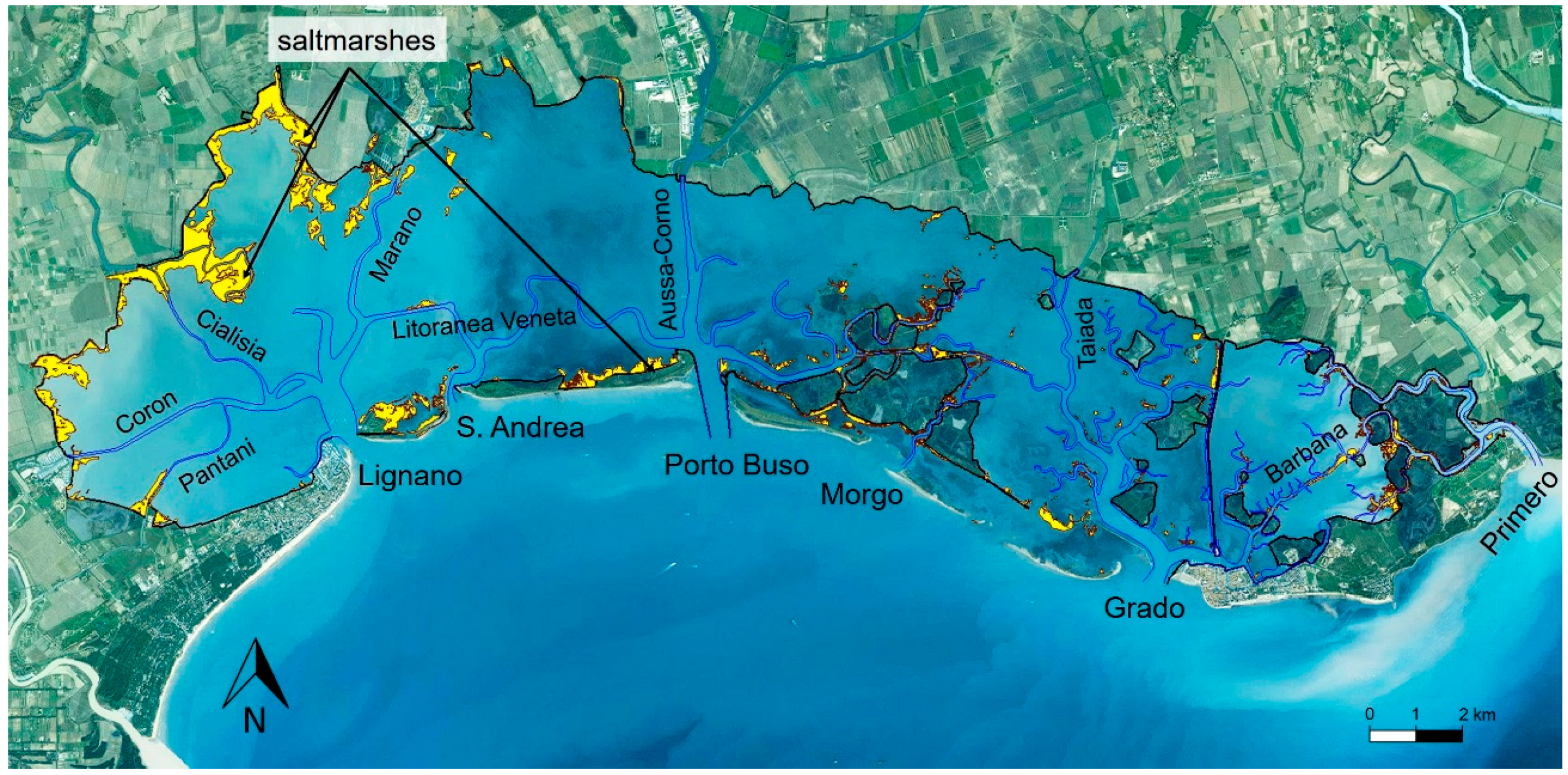
The study area is the Marano and Grado Lagoon, an extremely important coastal system between the low Friuli Venezia Giulia plain and the Northern Adriatic Sea, reproduced in Figure 1.
It roughly covers an area of 160 km2 bordered by the two deltas of Tagliamento river in the west and Isonzo river in the east; the lagoon extends parallel to the coastline along 32 km, while the mean distance between the internal edges and the barrier islands is about 5 km. Hydraulic circulation with the sea is guaranteed through six tidal inlets that interrupt the natural barrier island: Lignano, S. Andrea, Porto Buso, Morgo, Grado, and Primero. There are some rivers and channels flowing into the lagoon from its northern border, most of which are resurgence waters, with a total mean discharge of 70 m3/s [7]. The contribution of this fresh water input has hydrodynamic effects only localized at the mouth of the rivers itself and therefore in the innermost part of the lagoon [33]. For this reason, from the point of view of a global study, it has not been considered in the present work.
The computational grid of the morphological-hydrodynamic model covers the entire lagoon area and a portion of the sea strictly close to the lagoon inlets and barrier island, as depicted in Figure 2. The mesh consists of quadrangular elements, with a resolution variable from about 100 m in the tidal flats, and 2 m in the transverse direction of secondary channels. The choice of a structured mesh makes it possible to follow the flow in the channels better and to ensure a high resolution of the hydrodynamic variables.
SWAN, instead requires an unstructured triangular grid and the spatial domain is the same as the hydrodynamic, but limited to the lagoon extension; in fact, the offshore wave motion and the relative longshore currents and connected sediment transport have not been considered for the purpose of the present work, as only waves generated inside the lagoon have a role in the investigated process. The elements have a variable size from about 50 m and 15 m in the inner lagoon channels. Morphological and bathymetric features of the lagoon are known from a topographic survey carried out in 2011 [33,48] and subsequent detail taking of the main tidal inlets and channels. The mean depth of the lagoon is about 1 m.
A regular exchange grid with cell size of 50 m is used to interpolate wave and hydrodynamic results from each own module to the other. The sequential interaction is performed with an alternating time step set equal to Δtint = 900 s.
3.1. Hydrodynamic Settings
Hydrodynamic mesh boundaries have been plotted following the external embankments and barrier islands to reproduce the perimeter of the lagoon area. They represent hydraulically closed limits to which a wall boundary condition has been applied. Identical considerations can be made for the perimeter of fishing valleys and small islands placed inside the lagoon, excluded from the computational domain.
Four fan-shaped open boundaries were reproduced in the sea so as not to constrain the tidal levels directly at the six inlets and consequently leaving flow discharges free: the first includes the Lignano and St. Andrea inlets, the second one comprises the two inlets of Porto Buso and Morgo, the third is connected to Grado and the last one to the Primero channel. At the open sea boundaries, a level which changes over time can be assigned, according to tidal conditions.
A Manning’s coefficient has been set to each cell of the mesh, chosen from four roughness classes that have been identified to represent a different degree of current bottom shear stress: tidal channels, zones that are emerged or wet only by the high tide, mudflats and areas colonized by seagrass. For this purpose, we have referred to vegetation distribution inside the lagoon reported on a map edited in 2012 [49].
An iterative calibration process has been necessary to define the coefficient for each class of resistance and to establish the tidal wave characteristics at the open boundary in terms of amplitude and phase as only those measured by the tide gauge stations placed at the mouths are known. In this respect, a validation analysis had previously been carried out on the average annual levels calculated from the recordings of the 21 tide gauge stations distributed in the lagoon area, through the comparison and a cross–correlation between different instruments. This analysis has pointed out the difficulty of defining coherent benchmarks, despite the large deployment of tools used for monitoring.
The tide gauge placed at Grado inlet has the longest available time series; a comparative analysis applying a zero-crossing technique carried out over 24 years of recording from 1991 to 2014, shows a good agreement between the annual mean levels registered in Grado and those registered in Trieste (Molo Sartorio) and in Venice (Punta della Salute), both having a greater historicity. This conclusion supports the choice to use Grado tidal measurements as representative for the level imposed at the open boundary.
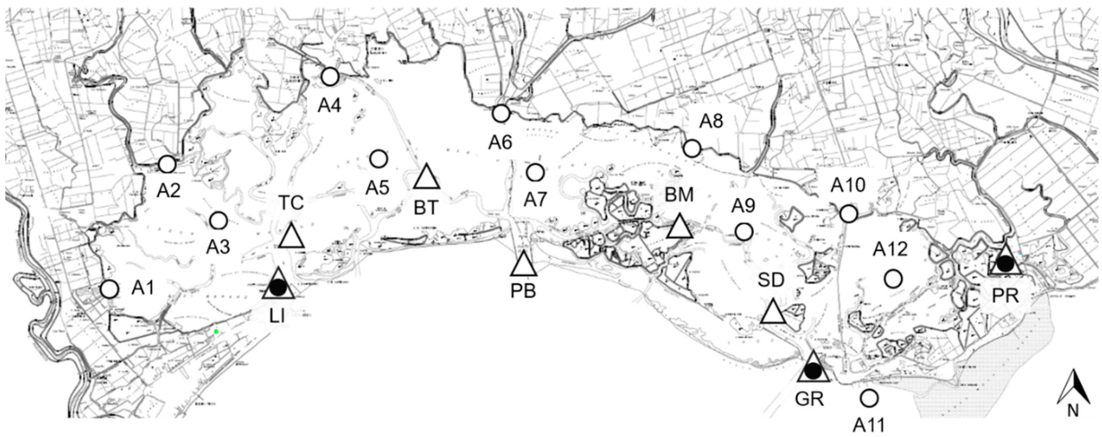
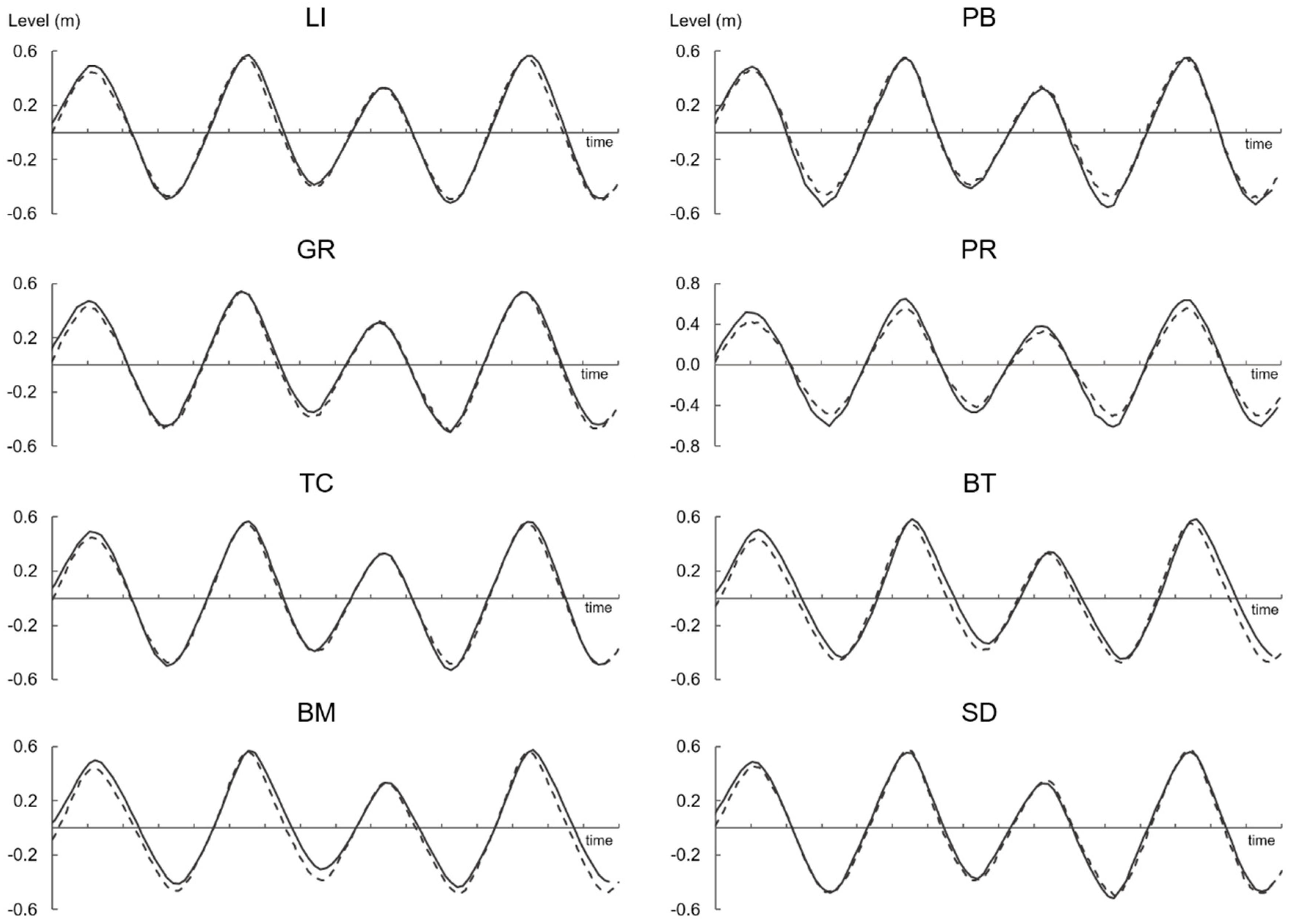
The simulated events refer to the period from 29 September 2014 to 3 October 2014, recorded at the same time from the largest number of active tide gauges present in the lagoon area, the displacement of which is depicted in Figure 3. The procedure was based on the best fitting between numerical results and measured level, minimizing the differences in both the amplitude and the phase of tidal waves, as shown in Figure 4.
In order to interpret the morphological evolution of the lagoon in the medium term, compatible with an annual extension, it has been important to establish appropriate conditions for tide and wind. These conditions should represent the forces acting in the lagoon over an average year from which both tidal currents and waves induced by wind depend directly.
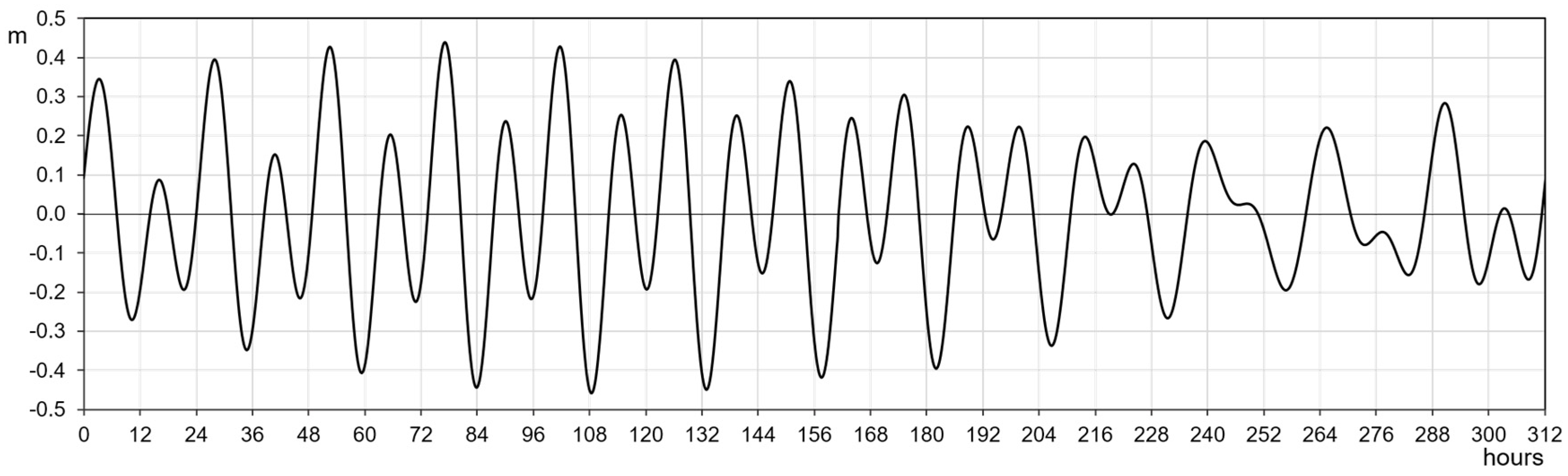
Using a Fast Fourier Transform algorithm, the annual spectra of signals, recorded by Grado’s tide gauge, were obtained both in terms of amplitude and phase. It is recognized that these spectra have three major peaks at the frequencies corresponding to the 12 h, 12.5 h, and 24 h, which are associated with the following harmonic constituents: the principal solar semidiurnal (S2), the principal lunar semidiurnal (M2) and the lunar diurnal (K1). From an ensemble analysis of the three frequency components, temporal mean amplitude and phase spectra were determined. Finally, applying the Inverse Fourier Transform, the signal for these average spectra was generated, which corresponds to the shape of the annual average tide searched for, that has a periodicity of 12.5 days, as it can be seen in Figure 5.
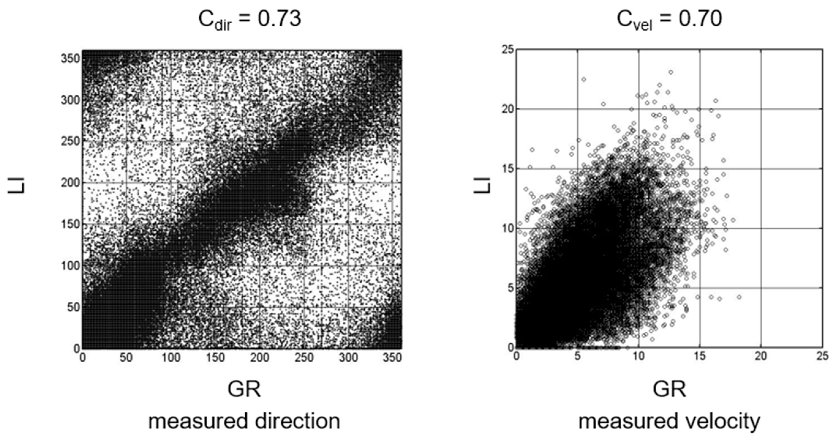
In addition to the tide levels, approximately 770,000 elements of wind data have been analyzed, some of these were recorded by the anemometers located inside the lagoon area and others were reconstructed by ARPA FVG (Regional Agency for the Environment Protection of Friuli Venezia Giulia), applying CALMET (CALifornia METeorological Model) [50] over a period between 2000 and 2014, whose position is indicated in Figure 3. A cross-correlation analysis between wind speed and directions measured by the two anemometers placed in Lignano and Grado has been conducted with the aim to check whether the wind is the same across the lagoon. The respective correlation coefficients indicate differences between the recordings in the two measurement poles, as can be seen from the data dispersion in the graphs shown in Figure 6.
A similar result has also been found in the cross-correlation analysis between reconstructed data. However, the correlation coefficients are very high among the points very close to the two respective anemometers (Table 1).
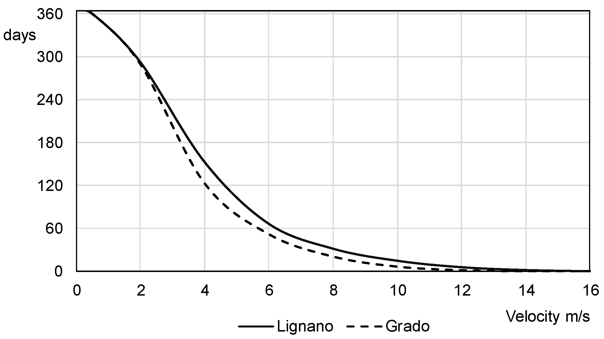
To verify if the winds recorded in Lignano and Grado also have different durations, the respective wind velocity duration curves were subsequently extrapolated, reporting for each wind speed the days in a year during which each speed is exceeded (Figure 7). The need to further sum up wind data, in order to derive an annual average anemometric characterization, has made it necessary to identify appropriate classes whose speed, direction and respective durations were estimated on the above-defined curves (Table 2). Considering that wind velocities above 14 m/s are recorded only for a few hours over the year, the speeds of 3 m/s, 6 m/s and 10 m/s have been chosen as representative for all wind data. Such representative velocities have been defined as barycentric ones of the areas subtended by the duration curves. We have found from the two curves similar durations to be assigned to each class, so we have finally decided to refer to average values. With the same approach used for wind speeds, four main sectors of directions have been defined to conduct an omnidirectional analysis, considering all potential effects a generic blowing wind would have on lagoon hydrodynamic variables. The representative directions of the four sectors are respectively: North, East, South and West.
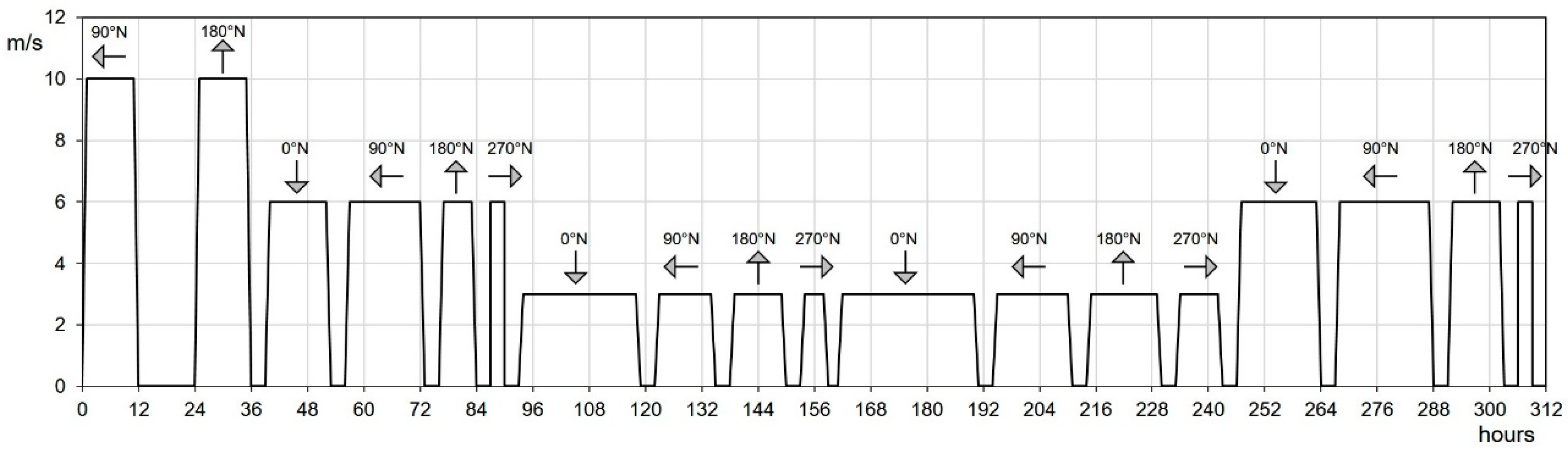
The last fundamental step has been to establish a suitable time sequence of the wind, both in terms of direction and intensity, on the annual average tide form. The duration of each wind intensity and direction has been calculated from the relative frequencies deriving from the above described analysis over a time span coinciding with the average tide periodicity. The different winds were alternated with distributed calm times; this sequence, represented in Figure 8, is the summary of the analyses of tidal and anemometric measurements and it establishes hydrodynamic forces acting in the lagoon over an average year; surface elevations, current velocities and bottom shear stress, which are responsible for the lifting and transport of sediments, depend on the conditions described above.
3.2. Morphodynamic Settings
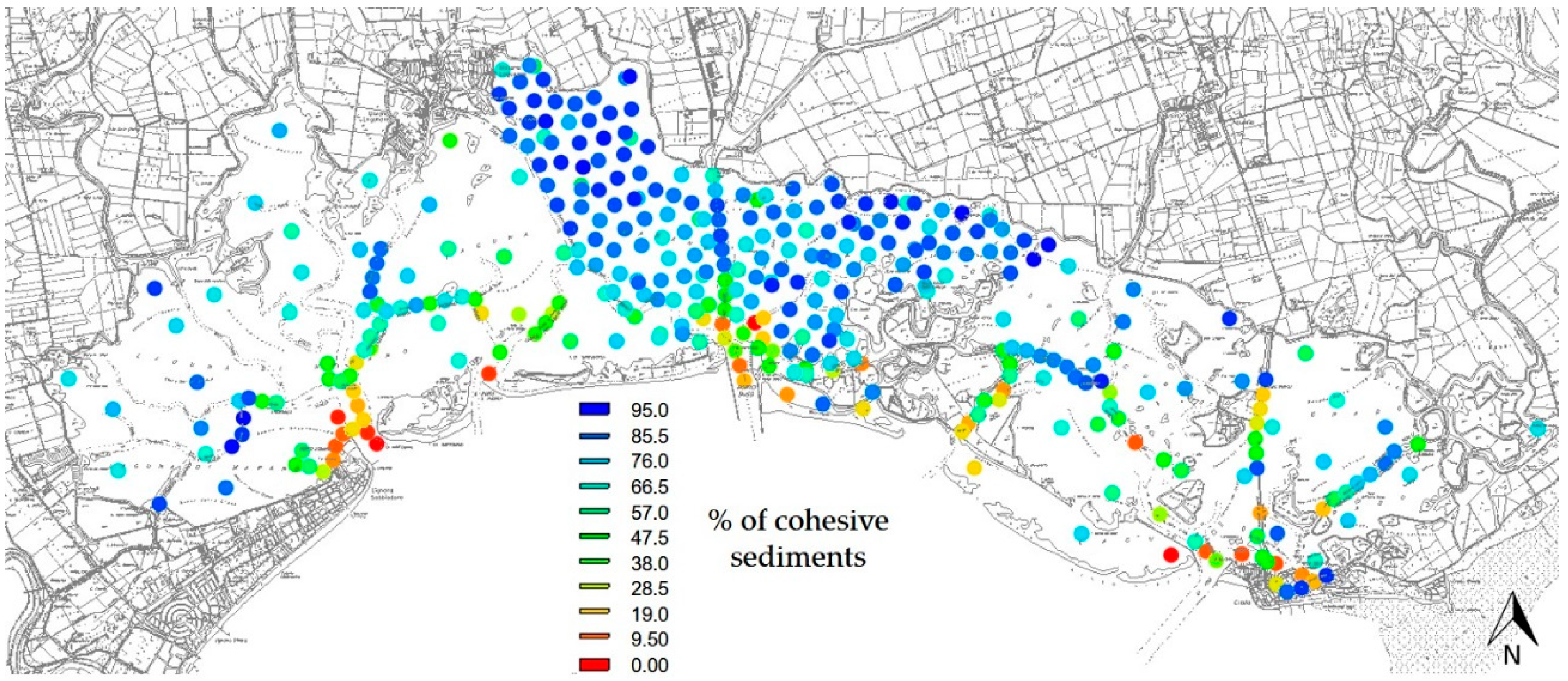
Sedimentological characteristics, in terms of representative diameter and percentage of cohesive and incoherent sediments are taken from measurement campaigns, carried out by ARPA FVG within the ICRAM (Central Institute for the Scientific Research and Technology Applied to the Sea) project over the last decade inside the entire lagoon area [51]. The lagoon sediments at the inlets are composed of calcareous sand. They become finer along the channels towards the inner part of the lagoon, where the percentage of silt and clay is quite close to 100%, as can be appreciated in Figure 9, which reports a synthesis of the data collected.
The morphological-hydrodynamic model distinguishes two grain-size classes of sediments: the granular sediments with a mean diameter set equal to 180 μm and the cohesive ones with a mean diameter set equal to 30 μm; these values were taken in agreement with the provided data.
To assign the threshold bed shear stress for the erosion of cohesive sediments there is no reference to known data for the lagoon of Marano and Grado. Laboratory tests with artificially deposited beds of natural muds have shown a great variability of the erosion threshold for a wide range of cohesive bed types, as a function of bed dry density and bulk density [31,32].
Furthermore, the morphological complexity of the lagoon leads to additional uncertainty about the choice of the critical shear stress values. In this regard, the lack of local measurements has resulted in a scrupulous work of comparison, by means of morphological similarity, with the critical shear stress values determined experimentally during several series of campaigns conducted within the Venice lagoon [30]. From these measurements, it is possible to detect a strong spatial and seasonal variability of the critical shear stress measured in several points in the lagoon and at different times of the year.
Based on these results and given the uncertainty in the correct attribution of the sedimentological parameters, we have chosen to adopt a morphological similarity criterion as follows. We have grouped the values obtained for the threshold bed shear stress inside the Venice lagoon, relating these values to common morphological structures. Specifically, it has been possible to recognize the following typologies: intertidal flats wet only by the high tide; permanently submerged mudflats; sites occupied by the seagrass in patches that covered 20–60% of the bed.
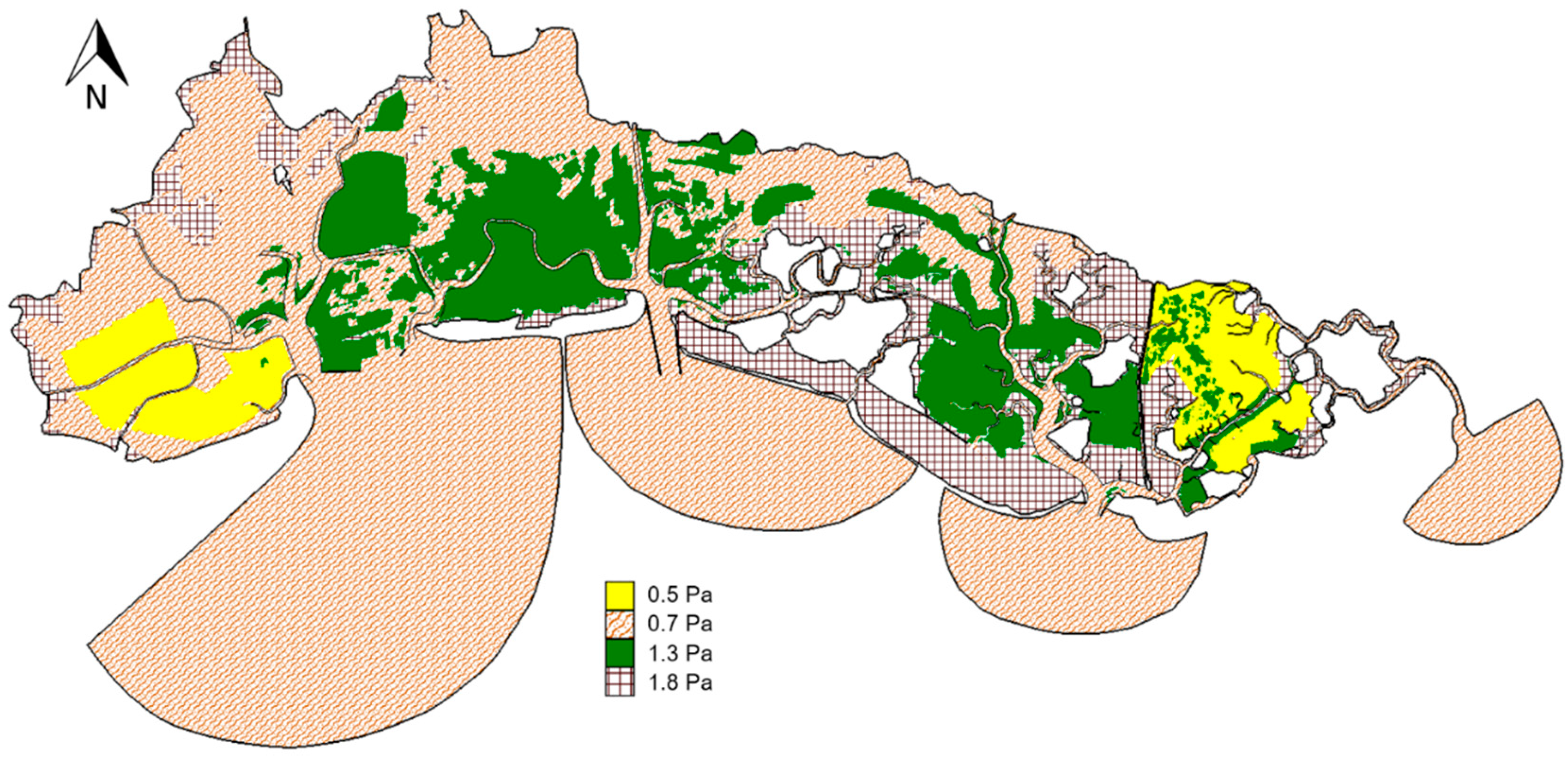
A similar characterization has been made for the morphologies typical of the lagoon of Marano and Grado to which we have assigned a representative mean value for the critical erosion shear stress, chosen from the available measurements, ranging from 0.7 Pa to 1.8 Pa. In addition to the three classes described above, it has been considered appropriate to introduce a fourth category, referring to the mudflats that, due to some causes, some of which are external, are subject to greater mobility of the cohesive sediment. This class is characterized by a lower critical erosion value, set equal to 0.5 Pa (Figure 10). It refers, for example, to areas used for shellfish farming, where the resuspension of sediments is comparable to that induced by the wave motion during storm conditions [52].
This procedure is innovative, as it differs from the traditional approaches in the morphodynamic study of lagoon or estuarine environments, which generally assume a single mean value of threshold bottom shear stress for the erosion of cohesive bed. To predict sediment transport and morphology over a period of one year, a morphological factor that allows you to amplify the variations of bottom height has been applied [53]. This factor has been set equal to 28 to simulate a time duration which coincides with the average tidal periodicity (Figure 8).
3.3. Spectral Model
In this study, SWAN has been run in stationary mode and it is set up for reproducing the refraction and shoaling induced by bottom and currents. The source terms included in the simulation take into account: the wave growth by wind and whitecapping according to Janssen [54]; the wave decay by bottom friction conforming to Madsen formulation [55] with an equivalent roughness length scale of the bottom of 0.05 m; depth-induced breaking with a constant breaking parameter equal to 0.78; quadruplet wave-wave interactions which are fundamental in the generation process. The lowest and the highest discrete frequency used in the calculation are respectively set equal to 0.071 Hz and 2 Hz. The spectral directions cover the full circle with a resolution of 6°.
4. Model Results and Discussion
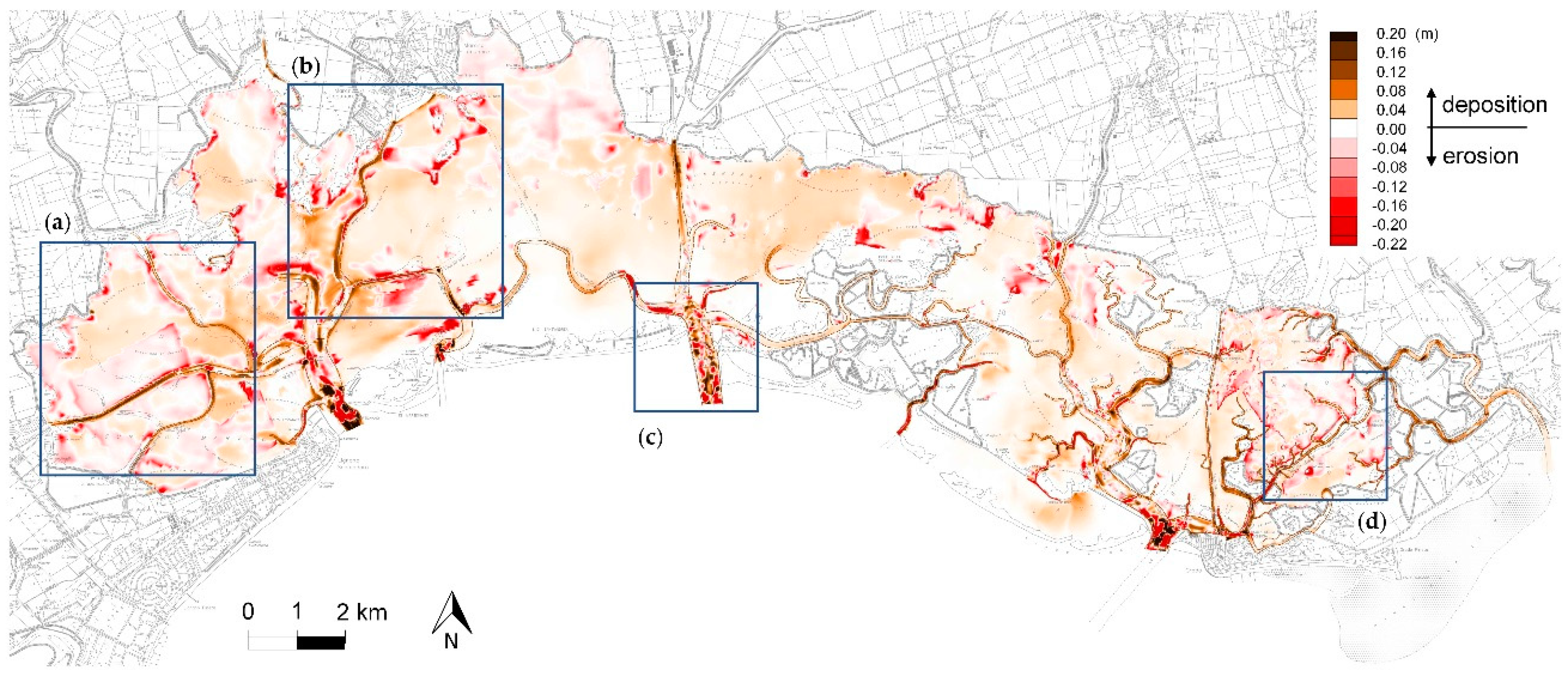
The morphological evolution of the lagoon over a period of an average year has been simulated. Numerical results of the coupled model have given the new bathymetries. Spatial distribution of erosion and deposits of sediment can be found from the differences between final and initial bed levels, as shown in Figure 11. The results confirm that the interaction between tidal currents and waves is the major hydrodynamic processes acting on intertidal flats. Most of the erosion areas are concentrated in the shallow depths of tidal flats and near saltmarshes, where the bottom shear stresses of wind waves are greater. A peculiarity which emerged from the analysis is the role played by the interaction between waves and currents that causes an increase of the bottom shear stresses mainly at the edge of the channels and at the intersection between different branches. The suspended sediment is entrained and carried by currents that pour the material into the network of channels. In this regard, we can observe that deposition of cohesive sediments occurs mainly inside channels and in particular along the branches that really require ordinary annual dredging interventions, as can be seen for example in the panels of Figure 11, the enlarged details of which are shown in Figure 12a–d.
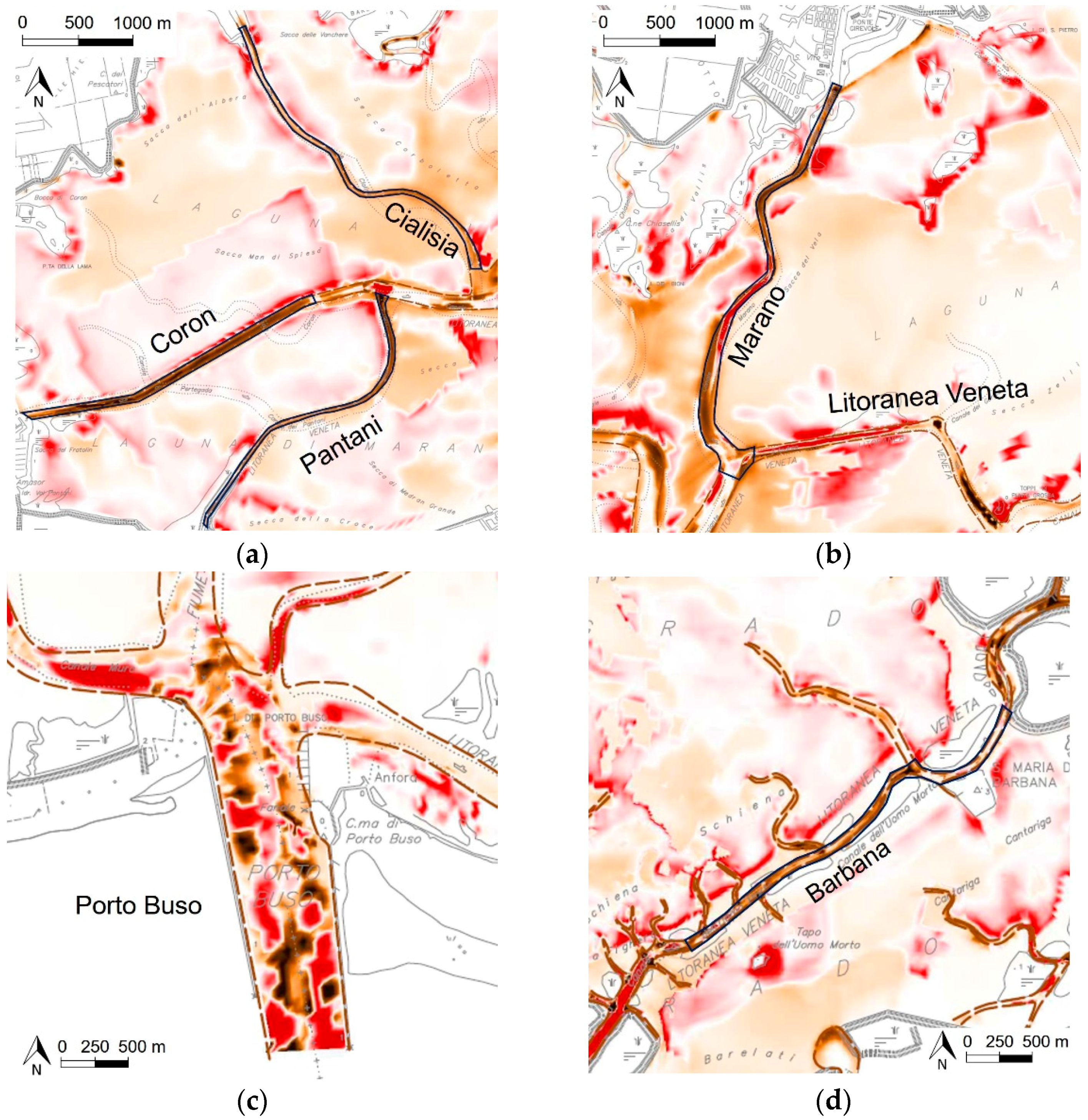
The transition between deposition and erosion is sometimes determined by a different critical erosion shear stress at the bottom (Figure 10) or by a change of bathymetry. As examples, the first case is that of the area adjacent to the north edge of the Coron channel (Figure 12a), reserved for shellfish farming, or even the south area of the Litoranea Veneta channel (Figure 12b), where phanerogams are dotted around and therefore stabilize the bottom only in some sections. The second case is that of the saltmarshes system of the area close to Marano and Barbana channels (Figure 12b,d), where the very shallow depths make the bed more exposed to wind wave erosion, as Fontolan et al. [33] have also observed.
At the lagoon inlets, such as that of Porto Buso, there is a continuous passage between erosions and depositions, due to strong vorticity of current velocities. Bearing in mind that to reproduce the morphology of a tidal inlet correctly it would also be necessary to consider the longshore currents and therefore the external wave motion, the results were however consistent with the very irregular nature of the bottom inside the deeper channels. At the present time, there are no bathymetric surveys carried out at short time intervals and our comparisons can only be qualitative.
The model is rather validated through the volumes dredged in the sections actually recognized as critical by the public administration. The numerical deposited volumes have therefore been calculated and compared with the average annual volume dredged on the basis of the field data. The correspondence between numerical values and dredged volumes, reported in Table 3, is really satisfactory and corroborates the numerical approach used to simulate morphodynamic changes due not just to a singular event, but a sequence of tides and winds representative of hydrodynamic forces acting over an average year.
In particular, it can be recognized that winds with a velocity of 10 m/s contribute significantly to cohesive sediment resuspension resulting in higher wave conditions; resuspension is followed subsequently by storage phases during calm events, which make it possible to reach a deposited volume inside selected channels equal, on average, to 75% of the total.
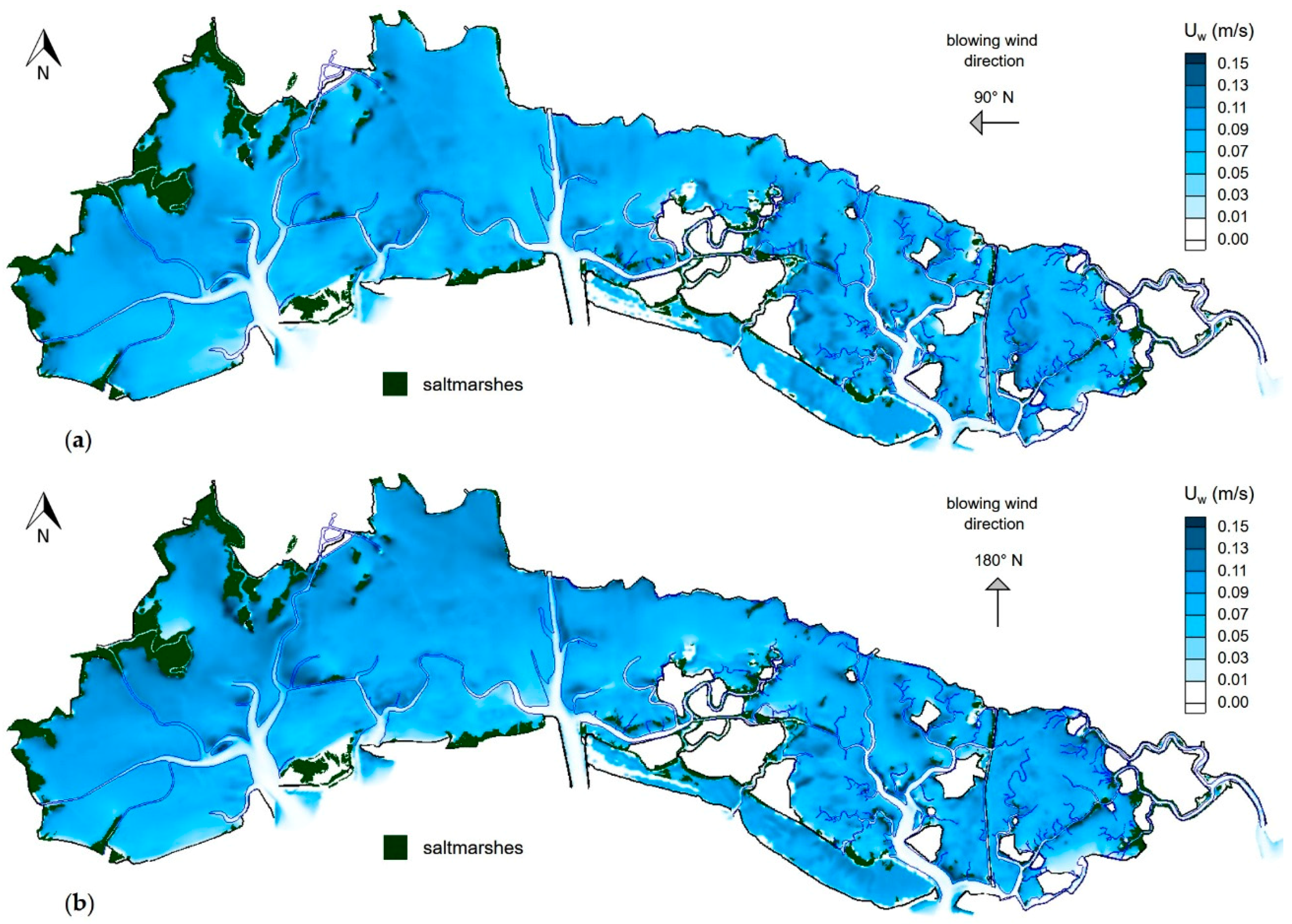
The maximum values of significant wave height, during most intense events, are included in the range of 0.3 ÷ 0.4 m. Both directions of Bora-Levante and Scirocco give comparable results in term of wave height and maximal bottom orbital velocity, despite the greater exposure of the lagoon basin to Bora-Levante sector. This is an important achievement that highlights the strongly nonlinear context due to the interaction with the bottom and the currents.
This complex interaction significantly affects the generation process of wind waves, which cannot be treated as in the case of deep waters and in particular when considering the fetch concept. Due to the lagoon morphology and the level variation that can expose some areas or submerge others one, even shorter free sea distances can give comparable wave motion characteristics as depicted in Figure 13a,b. Moreover, saturation is achieved in a very short time, approximately of one hour in all of the lagoon basin and the interaction with the bottom and the currents increases the phenomenon. This result further strengthened the choice to consider an omnidirectional distribution of winds, summed up in the four representative directions and not just the prevailing one.
Moderate or quiet winds produce lower wave orbital velocity that affect the sediment resuspension less, yet condition the lagoon hydrodynamic. Transverse flows are generated due to the wind shear stresses, the set-up of the water surface and the different discharges through the lagoon inlets.
Currents have a redistribution effect of cohesive sediments within the channels: the higher velocities in the main branches erode the silt and clay deposited during calm times and transport the material into secondary channels. Within the same channels there may be some stretches where the current velocities are quite high and clear the bottom, such happens along the Coron channel which requires annual dredging of only a critical stretch and not along its entire development until the confluence with Cialisia (Figure 12a) or along Litoranea Veneta channel (Figure 12a,b) where alternating erosion and deposition sections can be found.
In the simulation setup two grain size classes of sediments were considered. The obtained numerical results confirm that the sediment transport is totally cohesive on the tidal flats and along the inner shallow channels, while moving towards the lagoon inlets, through the branches with deeper water and stronger current velocities, there is also the contribution of granular sediment, which becomes predominant inside an area with a radius of about 1 km, close to the mouth. This is coherent with the cores carried out and used for the simulation setup depicted in Figure 9.
The important role of the interaction between waves and currents has been noted both in the generation process of wave motion and in the effects on sediment transport. As anticipated above, several authors limit interaction terms, neglecting current velocities and updating, in the wave model used, just the surface elevation according to tidal level as if current velocities have no effects on waves parameters. As already stated, in this simulation, a fully spectral model is used and takes as input from the hydrodynamic model both water levels and current velocities. To verify the validity of this approach in terms of sediment transport a similar simulation has been performed, with the same boundary conditions in terms of tide and winds and the same numerical parameters. The only difference is that the spectral model has generated waves only taking into account water levels and ignoring current velocities. The differences in morphodynamic results are important in the whole lagoon basin, above all in terms of the amount of erosion and deposits. A comparison between the deposited volumes of cohesive sediments, inside the channels mentioned above, with and without the full interaction, highlights this outcome (Table 3).
The comparison shows that the interactions between waves and currents, especially in a complex morphological and hydrodynamical context such as the lagoon, cannot be neglected or reduced.
5. Conclusions
A 2DH morphological—hydrodynamic and spectral coupled model has been applied to study the sediment transport in a transitional environment such a lagoon, where the interaction of wave motion with shallow bottoms and tidal currents is crucial. Given the morphological complexity of this domain, great attention has been taken to reproduce bathymetries and channel geometry, exploiting the computational efficiency of a shallow water model.
A new procedure to detect a sequence of winds and tides, that are representative of the hydrodynamic forces acting in the lagoon over an average year, has been presented. Using correlation techniques and spectral analysis of temporal signals, the average tide and wind distribution for different intensities and directions were reconstructed.
It has been verified that winds blowing from different directions with equal velocity can generate wave motion of comparable intensity despite the fetch being limited in size. This particular achievement emphasizes the importance of non-linear interaction between waves and currents. More intense winds generate wave motion that can mobilize the sediment from the tidal flats, while currents drag it. In this regard, lower winds contribute less to filling the channels but they still affect the overall lagoon hydrodynamics. The suspended load is deposited during calm period into channels.
The numerical volumes of cohesive sediments deposited in the critical branches of the lagoon match the real volumes annually dredged satisfactorily. This is an innovative result in state of the art numerical morphodynamic studies of lagoon and estuarine environments. The comparison of the new bathymetries at the end of simulation with the initial conditions confirms that most of the erosion areas are concentrated near saltmarshes and tidal flats, as pointed out in literature.
Another important element that differs from common approaches is the assumption of a spatially variable critical shear stress for the erosion of cohesive sediments, which takes into account the different morphologies and the presence of seagrass that has stabilizing effects on the bottom.
Among the future developments we intend to compare the numerical results obtained from the model on detailed bathymetric surveys taken at yearly distances.
Author Contributions
All the authors contributed equally to this work.
Funding
This research was co-funded by Regione Autonoma Friuli Venezia Giulia, Direzione centrale infrastrutture, mobilità, pianificazione territoriale, lavori pubblici e edilizia [CUP:D26D14000230002].
Conflicts of Interest
The authors declare no conflict of interest.
References
- Umgiesser, G.; Sclavo, M.; Carniel, S.; Bergamasco, A. Exploring the bottom shear stress variability in the Venice Lagoon. J. Mar. Syst. 2004, 51, 161–178. [Google Scholar] [CrossRef]
- Mariotti, G.; Fagherazzi, S. A numerical model for the coupled long-term evolution of salt marshes and tidal flats. J. Geophys. Res. 2010, 115, F01004. [Google Scholar] [CrossRef]
- Tonelli, M.; Petti, M. Numerical simulation of wave overtopping at coastal dikes and low-crested structures by means of a shock-capturing Boussinesq model. Coast. Eng. 2013, 79, 75–88. [Google Scholar] [CrossRef]
- Warner, J.C.; Sherwood, C.R.; Signell, R.P.; Harris, C.K.; Arango, H.G. Development of a three-dimensional, regional, coupled wave, current, and sediment-transport model. Comput. Geosci. 2008, 34, 1284–1306. [Google Scholar] [CrossRef]
- Nahon, A.; Bertin, X.; Fortunato, A.B.; Oliveira, A. Process-based 2DH morphodynamic modeling of tidal inlets: A comparison with empirical classifications and theories. Mar. Geol. 2012, 291, 1–11. [Google Scholar] [CrossRef]
- Carniello, L.; Defina, A.; D’Alpaos, L. Modeling sand-mud transport induced by tidal currents and wind waves in shallow microtidal basins: Application to the Venice Lagoon (Italy). Estuar. Coast. Shelf Sci. 2012, 102, 105–115. [Google Scholar] [CrossRef]
- Ferrarin, C.; Umgiesser, G.; Roland, A.; Bajo, M.; De Pascalis, F.; Ghezzo, M.; Scroccaro, I. Sediment dynamics and budget in a microtidal lagoon—A numerical investigation. Mar. Geol. 2016, 381, 163–174. [Google Scholar] [CrossRef]
- Ferrarin, C.; Cucco, A.; Umgiesser, G.; Bellafiore, D.; Amos, C.L. Modelling fluxes of water and sediment between Venice Lagoon and the sea. Cont. Shelf Res. 2010, 30, 904–914. [Google Scholar] [CrossRef] [Green Version]
- Gross, E.S.; MacWilliams, M.L.; Kimmerer, W.J. Three-dimensional modeling of tidal hydrodynamics in the San Francisco Estuary. San Franc. Estuary Watershed Sci. 2010, 7. [Google Scholar] [CrossRef]
- Villaret, C.; Hervouet, J.M.; Kopmann, R.; Merkel, U.; Davies, A.G. Morphodynamic modeling using the Telemac finite-element system. Comput. Geosci. 2013, 53, 105–113. [Google Scholar] [CrossRef]
- Tambroni, N.; Ferrarin, C.; Canestrelli, A. Benchmark on the numerical simulations of the hydrodynamic and morphodynamic evolution of tidal channels and tidal inlets. Cont. Shelf Res. 2010, 30, 963–983. [Google Scholar] [CrossRef]
- Mellor, G.L. The Depth-Dependent Current and Wave Interaction Equations: A Revision. J. Phys. Oceanogr. 2008, 38, 2587–2596. [Google Scholar] [CrossRef]
- Bennis, A.; Ardhuin, F. Comments on “The Depth-Dependent Current and Wave Interaction Equations: A Revision”. J. Phys. Oceanogr. 2011, 41, 2008–2012. [Google Scholar] [CrossRef]
- Booij, N.; Ris, R.C.; Holthuijsen, L.H. A third-generation wave model for coastal regions, Part I, Model description and validation. J. Geophys. Res. 1999, 104, 7649–7666. [Google Scholar] [CrossRef]
- Holthuijsen, L.H.; Booij, N.; Herbers, T.H.C. A prediction model for stationary, short crested waves in shallow water with ambient currents. Coast. Eng. 1989, 13, 23–54. [Google Scholar] [CrossRef]
- Sleigh, P.A.; Gaskell, P.H.; Berzins, M.; Wright, N.G. An unstructured finite-volume algorithm for predicting flow in rivers and estuaries. Comput. Fluids 1998, 27, 479–508. [Google Scholar] [CrossRef]
- Young, I.R. Wind Generated Ocean Waves; Elsevier: Oxford, UK, 1999. [Google Scholar]
- Longuet-Higgins, M.S.; Stewart, R.W. Changes in the form of short gravity waves on long waves and tidal currents. J. Fluid Mech. 1960, 8, 565–583. [Google Scholar] [CrossRef]
- Longuet-Higgins, M.S.; Stewart, R.W. Radiation stresses in water waves; A physical discussion, with applications. Deep Sea Res. Oceanogr. Abstr. 1964, 11, 529–562. [Google Scholar] [CrossRef]
- Whitham, G. Mass, momentum and energy flux in water waves. J. Fluid Mech. 1962, 12, 135–147. [Google Scholar] [CrossRef]
- Jonsson, I.G.; Skougaard, C.; Wang, J.D. Interaction between Waves and Currents. Coast. Eng. 1970, 1, 489–507. [Google Scholar] [CrossRef]
- Jonsson, I.G. Energy flux and wave action in gravity waves propagating on a current. J. Hydr. Res. 1978, 16, 223–234. [Google Scholar] [CrossRef]
- Carniello, L.; Defina, A.; Fagherazzi, S.; D’Alpaos, L. A combined wind wave–tidal model for the Venice lagoon, Italy. J. Geophys. Res. 2005, 110, F04007. [Google Scholar] [CrossRef]
- Phillips, O. On the dynamics of unsteady gravity waves of finite amplitude Part 1. The elementary interactions. J. Fluid Mech. 1960, 9, 193–217. [Google Scholar] [CrossRef]
- Hasselmann, K. On the non-linear energy transfer in a gravity-wave spectrum Part 1. General theory. J. Fluid Mech. 1962, 12, 481–500. [Google Scholar] [CrossRef]
- Bolaños-Sanchez, R.; Riethmüller, R.; Gayer, G.; Amos, C.L. Sediment Transport in a Tidal Lagoon Subject to Varying Winds Evaluated with a Coupled Current-Wave Model. J. Coast. Res. 2005, 21, e11–e26. [Google Scholar] [CrossRef]
- Plecha, S.; Silva, P.A.; Oliveira, A.; Dias, J.M. Establishing the wave climate influence on the morphodynamics of a coastal lagoon inlet. Ocean Dyn. 2012, 62, 799–814. [Google Scholar] [CrossRef]
- Van der Wegen, M.; Dastgheib, A.; Jaffe, B.E.; Roelvink, D. Bed composition generation for morphodynamic modeling: Case study of San Pablo Bay in California, USA. Ocean Dyn. 2010, 61, 173–186. [Google Scholar] [CrossRef]
- Fagherazzi, S.; Carniello, L.; D’Alpaos, L.; Defina, A. Critical bifurcation of shallow microtidal landforms in tidal flats and salt marshes. Proc. Natl. Acad. Sci. USA 2006, 103, 8337–8341. [Google Scholar] [CrossRef] [PubMed]
- Amos, C.L.; Bergamasco, A.; Umgiesser, G.; Cappucci, S.; Cloutier, D.; Denat, L.; Flindt, M.; Bonardi, M.; Cristante, S. The stability of tidal flats in Venice Lagoon—the results of in-situ measurements using two benthic, annular flumes. J. Mar. Syst. 2004, 51, 211–241. [Google Scholar] [CrossRef]
- Delo, E.; Ockenden, M.C. Estuarine Muds Manual; Technical Report SR 309; HR Wallingford Ltd.: Wallingford, UK, 1992. [Google Scholar]
- Mitchener, H.; Torfs, H.; Whitehouse, R. Erosion of mud/sand mixtures. Coast. Eng. 1996, 29, 1–25. [Google Scholar] [CrossRef]
- Fontolan, G.; Pillon, S.; Bezzi, A.; Villalta, R.; Lipizer, M.; Triches, A.; D’Aietti, A. Human impact and the historical transformation of saltmarshes in the Marano and Grado Lagoon, northern Adriatic Sea. Estuar. Coast. Shelf Sci. 2012, 113, 41–56. [Google Scholar] [CrossRef]
- Van Rijn, L.C. Principles of Sediment Transport in Rivers, Estuaries and Coastal Seas; Aqua Publications: Amsterdam, The Netherlands, 1993; 715p. [Google Scholar]
- Soulsby, R.L. Dynamics of Marine Sands: A Manual for Practical Applications; Thomas Telford Publications: London, UK, 1997; 249p. [Google Scholar]
- Van Rijn, L.C. Sediment transport, part II: Suspended load transport. J. Hydraul. Eng. 1984, 110. [Google Scholar] [CrossRef]
- Partheniades, E. Erosion and deposition of cohesive soils. J. Hydraul. Div. 1965, 91, 105–139. [Google Scholar]
- Teeter, A.M. Vertical Transport in Fine-Grained Suspension and Newly-Deposited Sediment. In Estuarine Cohesive Sediment Dynamics: Lecture Notes on Coastal and Estuarine Studies; Mehta, A.J., Ed.; Springer: New York, NY, USA, 1986; Volume 14. [Google Scholar]
- Whitehouse, R.J.S.; Soulsby, R.L.; Roberts, W.; Mitchener, H.J. Dynamics of Estuarine Muds; Technical Report; Thomas Telford: London, UK, 2000. [Google Scholar]
- Toro, E.F. Shock-Capturing Methods for Free-Surface Shallow Flows; John Wiley & Sons: New York, NY, USA, 2001. [Google Scholar]
- Audusse, E.; Bouchut, F.; Bristeau, M.-O.; Klein, R.; Perthame, B. A fast and stable well-balanced scheme with hydrostatic reconstruction for shallow water flows. SIAM J. Sci. Comput. 2004, 25, 2050–2065. [Google Scholar] [CrossRef]
- Liang, Q.; Marche, F. Numerical resolution of well-balanced shallow water equations with complex source terms. Adv. Water Resour. 2009, 32, 873–884. [Google Scholar] [CrossRef]
- Bosa, S.; Petti, M. A Numerical Model of the Wave that Overtopped the Vajont Dam in 1963. Water Resour. Manag. 2013, 27, 1763–1779. [Google Scholar] [CrossRef]
- Petti, M.; Bosa, S.; Pascolo, S.; Lubrano, F. Hydrodynamic Wave Effects on the River Delta: An Efficient 2HD Numerical Model. In Proceedings of the Fifteenth International Conference on Civil, Structural and Environmental Engineering Computing, Faculty of Civil Engineering, Czech Technical University of Prague, Prague, Czech Republic, 1–4 September 2015; CIVIL-COMP Press: Stirling, UK, 2015. [Google Scholar]
- Pascolo, S.; Petti, M.; Bosa, S. Wave–Current Interaction: A 2DH Model for Turbulent Jet and Bottom-Friction Dissipation. Water 2018, 10, 392. [Google Scholar] [CrossRef]
- Bosa, S.; Petti, M.; Lubrano, F.; Pascolo, S. Finite Volume Morphodynamic Model Useful in Coastal Environment. Procedia Eng. 2016, 161, 1887–1892. [Google Scholar] [CrossRef]
- Bosa, S.; Petti, M.; Lubrano, F.; Pascolo, S. Morphodynamic Model Suitable for River Flow and Wave-Current Interaction. IOP Conf. Ser. Mater. Sci. Eng. 2017, 245. [Google Scholar] [CrossRef]
- Triches, A.; Pillon, S.; Bezzi, A.; Lipizer, M.; Gordini, E.; Villalta, R.; Fontolan, G.; Menchini, G. Carta Batimetrica Della Laguna di Marano e Grado; Arti Grafiche Friulane, Imoco spa: Udine, Italy, 2011; 39p, 5 Maps; ISBN 978-88-95980-02-7. [Google Scholar]
- Boscutti, F.; Marcorin, I.; Sigura, M.; Bressan, E.; Tamberlich, F.; Vianello, A.; Casolo, V. Distribution modeling of seagrasses in brackish waters of Grado-Marano lagoon (Northern Adriatic Sea). Estuar. Coast. Shelf Sci. 2015, 164, 183–193. [Google Scholar] [CrossRef]
- Scire, J.S.; Insley, E.M.; Yamartino, R.J. Model Formulation and User’s Guide for the CALMET Meteorological Model; Sigma Research Corp.: Concord, MA, USA, 1990. [Google Scholar]
- ICRAM. Piano di Caratterizzazione Ambientale di Aree e Canali Interni Alla Laguna di Marano Lagunare e Grado, Sito di bonifica di interesse nazionale di Marano lagunare e Grado. Document CII–Pr–FVG–G M–07.03. 2008; Italy. (In Italian)
- Pranovi, F.; Da Ponte, F.; Raicevich, S.; Giovanardi, O. A multidisciplinary study of the immediate effects of mechanical clam harvesting in the Venice Lagoon. ICES J. Mar. Sci. 2004, 61, 43–52. [Google Scholar] [CrossRef]
- Roelvink, J.A. Coastal morphodynamic evolution techniques. Coast. Eng. 2006, 53, 277–287. [Google Scholar] [CrossRef]
- Janssen, P.A.E.M. Quasi-linear theory of wind-wave generation applied to wave forecasting. J. Phys. Oceanogr. 1991, 21, 1631–1642. [Google Scholar] [CrossRef]
- Madsen, O.S.; Poon, Y.-K.; Graber, H.C. Spectral wave attenuation by bottom friction: Theory. In Proceedings of the 21th International Conference Coastal Engineering, ASCE, Costa del Sol-Malaga, Spain, 20–25 June 1988; pp. 492–504. [Google Scholar]
Figure 1.
Marano and Grado Lagoon, Italy. The six tidal inlets, the main channels and saltmarshes are highlighted.
Figure 1.
Marano and Grado Lagoon, Italy. The six tidal inlets, the main channels and saltmarshes are highlighted.

Figure 2.
Computational domains used in the simulations: the morphological-hydrodynamic structured mesh reproducing Marano and Grado Lagoon and the regular exchange grid. The mesh of SWAN (Simulating WAves Nearshore) comprises only the lagoon extension.
Figure 2.
Computational domains used in the simulations: the morphological-hydrodynamic structured mesh reproducing Marano and Grado Lagoon and the regular exchange grid. The mesh of SWAN (Simulating WAves Nearshore) comprises only the lagoon extension.

Figure 3.
Displacement of data collected inside lagoon area: tide gauges (triangles), anemometric data reconstructed by weather model (empty circles), anemometers (full circles).
Figure 3.
Displacement of data collected inside lagoon area: tide gauges (triangles), anemometric data reconstructed by weather model (empty circles), anemometers (full circles).

Figure 4.
Calibration procedure: comparison of measured level (dashed line) and computed water levels at the stations (solid lines) in the period from 29 September 2014 to 3 October 2014.
Figure 4.
Calibration procedure: comparison of measured level (dashed line) and computed water levels at the stations (solid lines) in the period from 29 September 2014 to 3 October 2014.

Figure 5.
Sequence of the reconstructed annual average tidal level.

Figure 6.
Cross correlation analysis between wind data measured by Lignano and Grado anemometers.

Figure 7.
Wind velocity duration curves of Lignano e Grado.

Figure 8.
Sequence of winds used in the simulation to represent hydrodynamic forces acting in the lagoon over an average year. The arrows indicate the directions from which the wind blows.
Figure 8.
Sequence of winds used in the simulation to represent hydrodynamic forces acting in the lagoon over an average year. The arrows indicate the directions from which the wind blows.

Figure 9.
Sampling stations distribution which refers to the measurement campaigns carried out by ARPA FVG (Regional Agency for the Environment Protection of Friuli Venezia Giulia) over the last decade inside the lagoon area. Contours indicate the percentage of cohesive sediments (silt and clay).
Figure 9.
Sampling stations distribution which refers to the measurement campaigns carried out by ARPA FVG (Regional Agency for the Environment Protection of Friuli Venezia Giulia) over the last decade inside the lagoon area. Contours indicate the percentage of cohesive sediments (silt and clay).

Figure 10.
Classes of critical shear stress and assignment to lagoon area.

Figure 11.
Morphological evolution of the lagoon over a period of an average year with erosion and deposition areas. (a–d): panels shown in detail in Figure 12a–d.
Figure 11.
Morphological evolution of the lagoon over a period of an average year with erosion and deposition areas. (a–d): panels shown in detail in Figure 12a–d.

Figure 12.
Details of some channels of Figure 11: (a) Pantani, Coron and Cialisia; (b) Marano and Litoranea Veneta; (c) Porto Buso; (d) Barbana. The dashed lines represent the edge of the channels, solid lines identify the critical branches that really require ordinary annual dredging intervention. The contour legend is the same as Figure 11.

Figure 13.
Simulated maximum bottom orbital velocities for wave motion generated by wind blowing from: (a) East; (b) South.
Figure 13.
Simulated maximum bottom orbital velocities for wave motion generated by wind blowing from: (a) East; (b) South.


Table 1.
Correlation coefficients for wind velocities (Cvel) and directions (Cdir) obtained by means the cross-correlation analyses between reconstructed anemometric data.
Table 1.
Correlation coefficients for wind velocities (Cvel) and directions (Cdir) obtained by means the cross-correlation analyses between reconstructed anemometric data.
| Area | LI-PR | LI-GR | A5-A9 | |||||
|---|---|---|---|---|---|---|---|---|
| west–east | Cvel | 0.73 | 0.58 | 0.81 | ||||
| Cdir | 0.71 | 0.77 | 0.87 | |||||
| LI-A1 | LI-A2 | LI-A3 | LI-A5 | A5-A4 | A5-A6 | A5-A7 | ||
| west | Cvel | 0.99 | 0.98 | 1.00 | 0.99 | 0.99 | 0.98 | 0.97 |
| Cdir | 0.99 | 0.98 | 1.00 | 0.99 | 0.99 | 0.97 | 0.97 | |
| GR-A9 | GR-A11 | GR-A10 | A8-A9 | A9-A10 | GR-PR | |||
| east | Cvel | 0.94 | 1.00 | 0.82 | 0.98 | 0.99 | 0.81 | |
| Cdir | 0.98 | 1.00 | 0.98 | 0.99 | 0.99 | 0.92 |
Table 2.
Identification of wind classes: representative speeds and respective durations calculated over 1 year. The last four columns represent the subdivision in percentage of days for the main chosen directions.
Table 2.
Identification of wind classes: representative speeds and respective durations calculated over 1 year. The last four columns represent the subdivision in percentage of days for the main chosen directions.
| Interval (m/s) | Representative Speed (m/s) | Duration (Days/Year) | Duration (% of Days/Year) | |||
|---|---|---|---|---|---|---|
| 0°–360° N | 0° N | 90° N | 180° N | 270° N | ||
| 0–2 | 0 | 74 | - | - | - | - |
| 2–4 | 3 | 152.5 | 18.3 | 9.7 | 8.6 | 5.3 |
| 4–8 | 6 | 112 | 10.1 | 11.9 | 6.7 | 2.0 |
| 8–14 | 10 | 26.5 | 1.3 | 4.1 | 1.7 | 0.1 |
Table 3.
Comparison between the simulated deposited volumes (m3) of cohesive sediments with and without the interaction between waves and current velocities with the average annual dredged volumes and the percentage differences between the two simulations.
Table 3.
Comparison between the simulated deposited volumes (m3) of cohesive sediments with and without the interaction between waves and current velocities with the average annual dredged volumes and the percentage differences between the two simulations.
| Channel | Average Annual Dredged Volumes | Simulated Volumes with Interaction | Simulated Volumes without Interaction | Percentage Difference |
|---|---|---|---|---|
| Cialisia | 8600 | 9400 | 6200 | −34% |
| Coron | 21,750 | 21,350 | 16,230 | −24% |
| Pantani | 9800 | 8450 | 5260 | −38% |
| Barbana | 4700 | 3900 | 3770 | −3% |
| Marano | 11,050 | 11,060 | 4500 | −59% |
© 2018 by the authors. Licensee MDPI, Basel, Switzerland. This article is an open access article distributed under the terms and conditions of the Creative Commons Attribution (CC BY) license (http://creativecommons.org/licenses/by/4.0/).
Share and Cite
MDPI and ACS Style
Petti, M.; Bosa, S.; Pascolo, S. Lagoon Sediment Dynamics: A Coupled Model to Study a Medium-Term Silting of Tidal Channels. Water 2018, 10, 569. https://doi.org/10.3390/w10050569
AMA Style
Petti M, Bosa S, Pascolo S. Lagoon Sediment Dynamics: A Coupled Model to Study a Medium-Term Silting of Tidal Channels. Water. 2018; 10(5):569. https://doi.org/10.3390/w10050569
Chicago/Turabian StylePetti, Marco, Silvia Bosa, and Sara Pascolo. 2018. "Lagoon Sediment Dynamics: A Coupled Model to Study a Medium-Term Silting of Tidal Channels" Water 10, no. 5: 569. https://doi.org/10.3390/w10050569
Note that from the first issue of 2016, this journal uses article numbers instead of page numbers. See further details here.