A Case Study for the Application of an Operational Two-Dimensional Real-Time Flooding Forecasting System and Smart Water Level Gauges on Roads in Tainan City, Taiwan


Abstract
:
1. Introduction
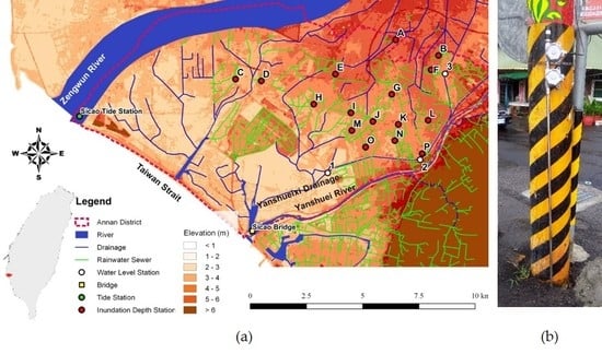
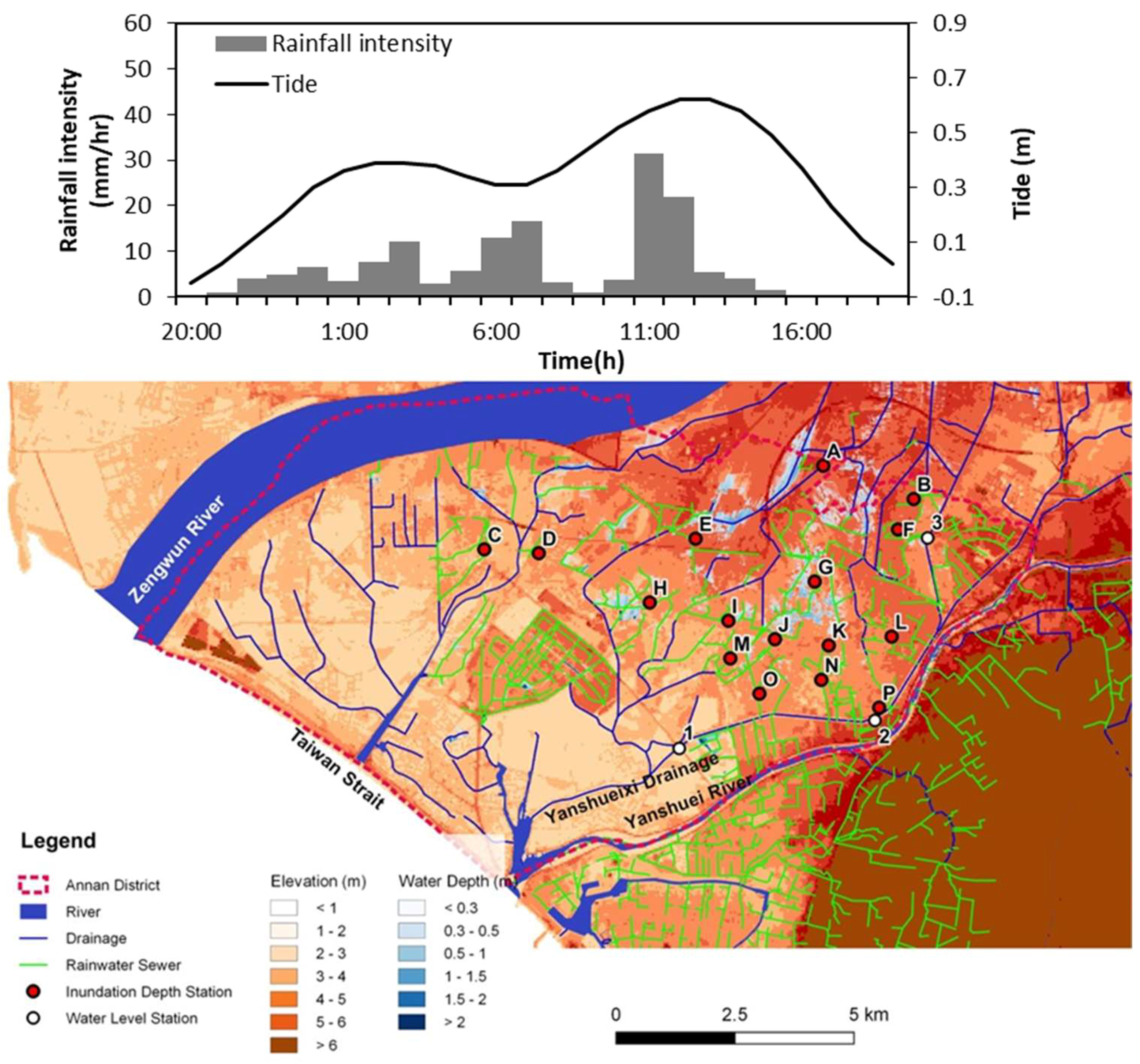
2. Study Area
3. Materials and Methods
3.1. Two-Dimensional Real-Time Flood Forecasting System
3.2. Field Observation
3.3. Statistical Error Indices of 1D Water Depth
3.4. Statistical Error Indices of 2D Inundation Depth
3.5. Performance Indicators
4. Results and Discussion
4.1. Water Level Stations
4.2. Inundation Depth Stations
4.3. Performance Indicators
4.4. The Causes of Uncertainties of the Two-Dimensional Real-Time Flood Forecasting System
4.5. The Application of Smart Water Level Gauges
5. Conclusions
Author Contributions
Funding
Acknowledgments
Conflicts of Interest
References
- Vehviläinen, B.; Huttunen, M. Hydrological forecasting and real time monitoring in Finland: The watershed simulation and forecasting system (WSFS). Water Qual. Meas. 2001. [Google Scholar] [CrossRef]
- Kirby, D. Flood integrated decision support system for Melbourne (FIDSS). In Proceedings of the 2015 Floodplain Management Association National Conference, Brisbane, Australian, 19–22 May 2015. [Google Scholar]
- Johnell, A.; Lindström, G.; Olsson, J. Deterministic evaluation of ensemble streamflow predictions in Sweden. Hydrol. Res. 2007, 38, 441–450. [Google Scholar] [CrossRef]
- Tospornsampan, M.J.; Malone, T.; Katry, P.; Pengel, B.; An, H.P. FMMP component 1 short and medium-term flood forecasting at the regional flood management and mitigation centre. Mekong River Comm. 2009, 7, 155–164. [Google Scholar]
- Werner, M.; Cranston, M.; Harrison, T.; Whitfield, D.; Schellekens, J. Recent developments in operational flood forecasting in England, Wales and Scotland. Meteorol. Appl. 2009, 16, 13–22. [Google Scholar] [CrossRef]
- Krajewski, W.F.; Ceynar, D.; Demir, I.; Goska, R.; Kruger, A.; Langel, C.; Mantilla, R.; Niemeier, J.; Quintero, F.; Seo, B.-C. Real-time flood forecasting and information system for the state of Iowa. Bull. Am. Meteorol. Soc. 2017, 98, 539–554. [Google Scholar] [CrossRef]
- Chang, C.-H. Establishment and Application of Radar Data and Hydrologic Models in an Integrated Platform of Hydrometeorology Observation; Water Resources Agency: Taichung, Taiwan, 2013.
- Chang, C.-H. The Development of Value-Add Application for Rainfall Rader Data and Multiple Hydrology Models Based on Fews_Taiwan; Water Resources Agency: Taichung, Taiwan, 2014.
- Syme, W.; Pinnell, M.; Wicks, J. Modelling flood inundation of urban areas in the UK using 2D/1D hydraulic models. In Proceedings of the 8th National Conference on Hydraulics in Water Engineering, Surfers Paradise, Australia, 13–16 July 2004. [Google Scholar]
- Chang, C.-H. Integrated Platform for Application of High-Performance 2D Inundation Simulation; Water Resources Planning Institute: Taichung, Taiwan, 2016.
- Hunter, N.M.; Bates, P.D.; Horritt, M.S.; Wilson, M.D. Simple spatially-distributed models for predicting flood inundation: A review. Geomorphology 2007, 90, 208–225. [Google Scholar] [CrossRef]
- Blumberg, A.F.; Georgas, N.; Yin, L.; Herrington, T.O.; Orton, P.M. Street-scale modeling of storm surge inundation along the New Jersey Hudson river waterfront. J. Atmos. Ocean. Technol. 2015, 32, 1486–1497. [Google Scholar] [CrossRef]
- Yin, J.; Yu, D.; Wilby, R. Modelling the impact of land subsidence on urban pluvial flooding: A case study of downtown Shanghai, China. Sci. Total Environ. 2016, 544, 744–753. [Google Scholar] [CrossRef] [PubMed] [Green Version]
- Liu, L.; Liu, Y.; Wang, X.; Yu, D.; Liu, K.; Huang, H.; Hu, G. Developing an Effective 2-D Urban Flood Inundation Model for City Emergency Management Based on Cellular Automata; Loughborough University: Loughborough, UK, 2015. [Google Scholar]
- Chang, T.-J.; Wang, C.-H.; Chen, A.S. A novel approach to model dynamic flow interactions between storm sewer system and overland surface for different land covers in urban areas. J. Hydrol. 2015, 524, 662–679. [Google Scholar] [CrossRef] [Green Version]
- Werner, M.; van Dijk, M.; Schellekens, J. Delft-fews: An open shell flood forecasting system. In Hydroinformatics; In 2 Volumes, with CD-ROM; World Scientific: Singapore, 2004; pp. 1205–1212. [Google Scholar]
- Werner, M.; Heynert, K. Open model integration—A review of practical examples in operational flood forecasting. In Proceedings of the Seventh International Conference on Hydroinformatics, Nice, France, 4–8 September 2006; pp. 155–162. [Google Scholar]
- Werner, M.; Schellekens, J.; Gijsbers, P.; van Dijk, M.; van den Akker, O.; Heynert, K. The Delft-FEWS flow forecasting system. Environ. Model. Softw. 2013, 40, 65–77. [Google Scholar] [CrossRef]
- Deltares. SOBEK User Manual; Deltares: Delft, The Netherlands, 2017. [Google Scholar]
- Doong, D.-J.; Lo, W.; Vojinovic, Z.; Lee, W.-L.; Lee, S.-P. Development of a new generation of flood inundation maps—A case study of the coastal city of Tainan, Taiwan. Water 2016, 8, 521. [Google Scholar] [CrossRef]
- Chiou, P.T.-K.; Chen, C.-R.; Chang, P.-L.; Jian, G.-J. Status and outlook of very short range forecasting system in Central Weather Bureau, Taiwan. In Applications with Weather Satellites II; International Society for Optics and Photonics: Bellingham, WA, USA, 2005; pp. 185–197. [Google Scholar]
- Wang, Y.; Zhang, J.; Chang, P.-L.; Langston, C.; Kaney, B.; Tang, L. Operational C-band dual-polarization radar QPE for the subtropical complex terrain of Taiwan. Adv. Meteorol. 2016, 2016. [Google Scholar] [CrossRef]
- Nash, J.E.; Sutcliffe, J.V. River flow forecasting through conceptual models part I—A discussion of principles. J. Hydrol. 1970, 10, 282–290. [Google Scholar] [CrossRef]
- Aronoff, S. Classification accuracy: A user approach. Photogramm. Eng. Remote Sens. 1982, 48, 1299–1307. [Google Scholar]
- Congalton, R.G. A review of assessing the accuracy of classifications of remotely sensed data. Remote Sens. Environ. 1991, 37, 35–46. [Google Scholar] [CrossRef]
- Purnami, S.W.; Zain, J.M.; Embong, A. A new expert system for diabetes disease diagnosis using modified spline smooth support vector machine. In Proceedings of the International Conference on Computational Science and Its Applications, Fukuoka, Japan, 23–26 March 2010; Springer: Berlin/Heidelberg, Germany, 2010; pp. 83–92. [Google Scholar]
- Wu, S.-J.; Lien, H.-C.; Chang, C.-H.; Shen, J.-C. Real-time correction of water stage forecast during rainstorm events using combination of forecast errors. Stoch. Environ. Res. Risk Assess. 2012, 26, 519–531. [Google Scholar] [CrossRef]
- Shen, D.; Wang, J.; Cheng, X.; Rui, Y.; Ye, S. Integration of 2-D hydraulic model and high-resolution lidar-derived DEM for floodplain flow modeling. Hydrol. Earth Syst. Sci. 2015, 19, 3605–3616. [Google Scholar] [CrossRef]


| Simulation | Observation | |
|---|---|---|
| Positive | Negative | |
| Positive | True positive (TP) | False positive (FP) |
| Negative | False negative (FN) | True negative (TN) |
| Rainfall Events | Station | Coefficient of Efficiency CE | Root Mean Square Error RMSEh (m) | Error of Peak Water Depth EHp (%) | Error of Time to Peak Water Depth ETh,p (min) |
|---|---|---|---|---|---|
| Storm 0611 | 1 | 0.686 | 0.19 | 8.9 | −60 |
| 2 | 0.716 | 0.27 | 20.7 | 30 | |
| 3 | 0.861 | 0.25 | 11.6 | 20 | |
| Typhoon Megi | 1 | 0.890 | 0.21 | −2.0 | 30 |
| 2 | 0.944 | 0.19 | 2.8 | 30 | |
| 3 | 0.957 | 0.21 | 5.9 | 10 |
| Rainfall Events | Station | Correlation Coefficient R | Root Mean Square Error RMSEd (m) | Error of Peak Inundation Depth EDp (m) | Error of Time to Peak Inundation Depth ETd,p (min) |
|---|---|---|---|---|---|
| Storm 0611 | E | 0.998 | 0.001 | 0.01 | 10 |
| J | 0.991 | 0.002 | 0.01 | 0 | |
| M | 0.639 | 0.026 | −0.06 | 10 | |
| P * | - | - | −0.11 | - | |
| Typhoon Megi | D | 0.982 | 0.007 | 0 | 10 |
| F | 0.909 | 0.012 | −0.06 | 30 | |
| G | 0.187 | 0.021 | −0.06 | 180 | |
| I | 0.998 | 0.001 | 0 | 0 | |
| J | 0.996 | 0.007 | 0 | 0 | |
| K | 0.943 | 0.028 | −0.03 | 10 |
| Simulation | Observation | |
|---|---|---|
| Positive | Negative | |
| Positive | 8 (TP) | 0 (FP) |
| Negative | 2 (FN) | 8 (TN) |
© 2018 by the authors. Licensee MDPI, Basel, Switzerland. This article is an open access article distributed under the terms and conditions of the Creative Commons Attribution (CC BY) license (http://creativecommons.org/licenses/by/4.0/).
Share and Cite
Chang, C.-H.; Chung, M.-K.; Yang, S.-Y.; Hsu, C.-T.; Wu, S.-J. A Case Study for the Application of an Operational Two-Dimensional Real-Time Flooding Forecasting System and Smart Water Level Gauges on Roads in Tainan City, Taiwan. Water 2018, 10, 574. https://doi.org/10.3390/w10050574
Chang C-H, Chung M-K, Yang S-Y, Hsu C-T, Wu S-J. A Case Study for the Application of an Operational Two-Dimensional Real-Time Flooding Forecasting System and Smart Water Level Gauges on Roads in Tainan City, Taiwan. Water. 2018; 10(5):574. https://doi.org/10.3390/w10050574
Chicago/Turabian StyleChang, Che-Hao, Ming-Ko Chung, Song-Yue Yang, Chih-Tsung Hsu, and Shiang-Jen Wu. 2018. "A Case Study for the Application of an Operational Two-Dimensional Real-Time Flooding Forecasting System and Smart Water Level Gauges on Roads in Tainan City, Taiwan" Water 10, no. 5: 574. https://doi.org/10.3390/w10050574