Top-Down and Bottom-Up Approaches for Water-Energy Balance in Portuguese Supply Systems


1
Civil Engineering Research and Innovation for Sustainability (CERIS), Instituto Superior Técnico, Universidade de Lisboa, Lisbon 1049-001, Portugal
2
Hydraulics Department, National Civil Engineering Laboratory, Lisbon 1700-066, Portugal
*
Author to whom correspondence should be addressed.
Water 2018, 10(5), 577; https://doi.org/10.3390/w10050577
Submission received: 28 March 2018
/
Revised: 20 April 2018
/
Accepted: 24 April 2018
/
Published: 28 April 2018
(This article belongs to the Special Issue Energy Efficient Management of Water Collection, Treatment, Storage and Distribution)
Abstract
:Water losses are responsible for increased energy consumption in water supply systems (WSS). The energy associated with water losses (EWL) is typically considered to be proportional to the water loss percentage obtained in water balances. However, this hypothesis is yet to be proved since flow does not vary linearly with headlosses in WSS. The aim of this paper is to validate the hypothesis, present real-life values for water-energy balance (WEB) components, and reference values for the key performance indicator that represents the ratio of total energy in excess (E3). This validation is achieved through the application of two approaches—top-down and bottom-up. The first approach requires minimum data, gives an overview of the main WEB components, and provides an effective diagnosis of energy inefficiencies through the calculation of E3 related to pumps, water losses, and networks. The second approach requires calibrated hydraulic models and provides a detailed assessment of the WEB components. Results allow the validation of the stated hypothesis as well as show that the most significant energy inefficiencies are associated with surplus energy, pumping, and water losses, each reaching up to 40% of total input energy. Less significant components are pipe friction and valve headlosses, each reaching up to 15% of total input energy.
1. Introduction
The water-energy nexus in the context of water supply systems (WSS) means that every drop of water has an embedded potential energy (natural, shaft, or mixed) and, therefore, water losses inevitably mean increased energy consumption. Energy costs are the second highest expenditure of a water utility after personnel [1]. Given the climate change challenges, particularly the increasingly more frequent droughts and floods worldwide, one of the main concerns of water utilities is to reduce water losses [2,3,4,5]. Water-energy consumption in WSS is context-dependent. Groundwater-based supply systems are generally more energy intensive than surface water-based systems because of higher pumping needs for water extraction. Each cubic meter of water loss has an embedded energy of 0.42 kWh for a median utility in the United States [6], 0.25 kWh/m3 in Brazil [7], and 0.14 kWh/m3 in Portugal [8].
Due to the water-energy nexus, an increase in water losses will necessary result in an increase in energy consumption. For instance, in groundwater systems, every additional unit of water (increased consumption and/or losses) will require more energy since the groundwater tables go down when more water is pumped up. On the other hand, solutions that reduce water losses will also have a positive impact on energy consumption [9]. For instance, reducing overflows in service tanks reduces both water losses and energy consumption as less water needs to be treated and pumped (in the case of rising or mixed systems). Mapping energy consumption through an energy-balance scheme for the water supply systems is useful to identify critical components requiring action and to plan intervention for improved energy efficiency.
Previous studies have addressed conceptual energy balances [10,11] with hardly any applications to real water supply systems without hydraulic models [12,13]. Top-down and bottom-up approaches for water-energy balance (WEB) were presented in [14]. The top-down approach requires minimum data (no hydraulic model is needed) and provides an effective diagnosis of energy inefficiencies in WSS. The bottom-up approach allows for the calculation of all energy balance components, but this is more data-demanding and most utilities do not have their networks modelled. The main hypothesis of the top-down approach is that the energy associated with water losses in a given WSS is proportional to the percentage of water losses provided by the water balance. This may not always be true—depending on the flow regime, headlosses can vary in a second-order degree with flow. Since the validation of this hypothesis has not been carried out yet, the primary objective of this paper is to do so.
The secondary objective of this paper, also a key innovative component, is to provide a range of real-life values for each energy balance component and reference values for E3, an energy performance indicator that helps in identifying main energy inefficiencies. The bottom-up approach has been applied in a large dataset of water supply systems in Portugal and results have been compared with the top-down approach. This dataset has been collected during a Portuguese collaborative project (iPerdas), through which 17 water utilities have developed master plans for controlling water losses and improving energy efficiency [15]. Two different methods have been applied to estimate the dissipated energy associated with headlosses and water losses. The first method (M1) assumes that water losses are distributed proportionally to network flow and involves the calculation of two simulations (with and without water losses); these calculations have been carried out as defined in [7]. The second method (M2) assumes that (real) water losses are proportional to pressure and to the length of pipes confluent to each node, and so, require the redistribution of water losses accordingly.
2. Methodology
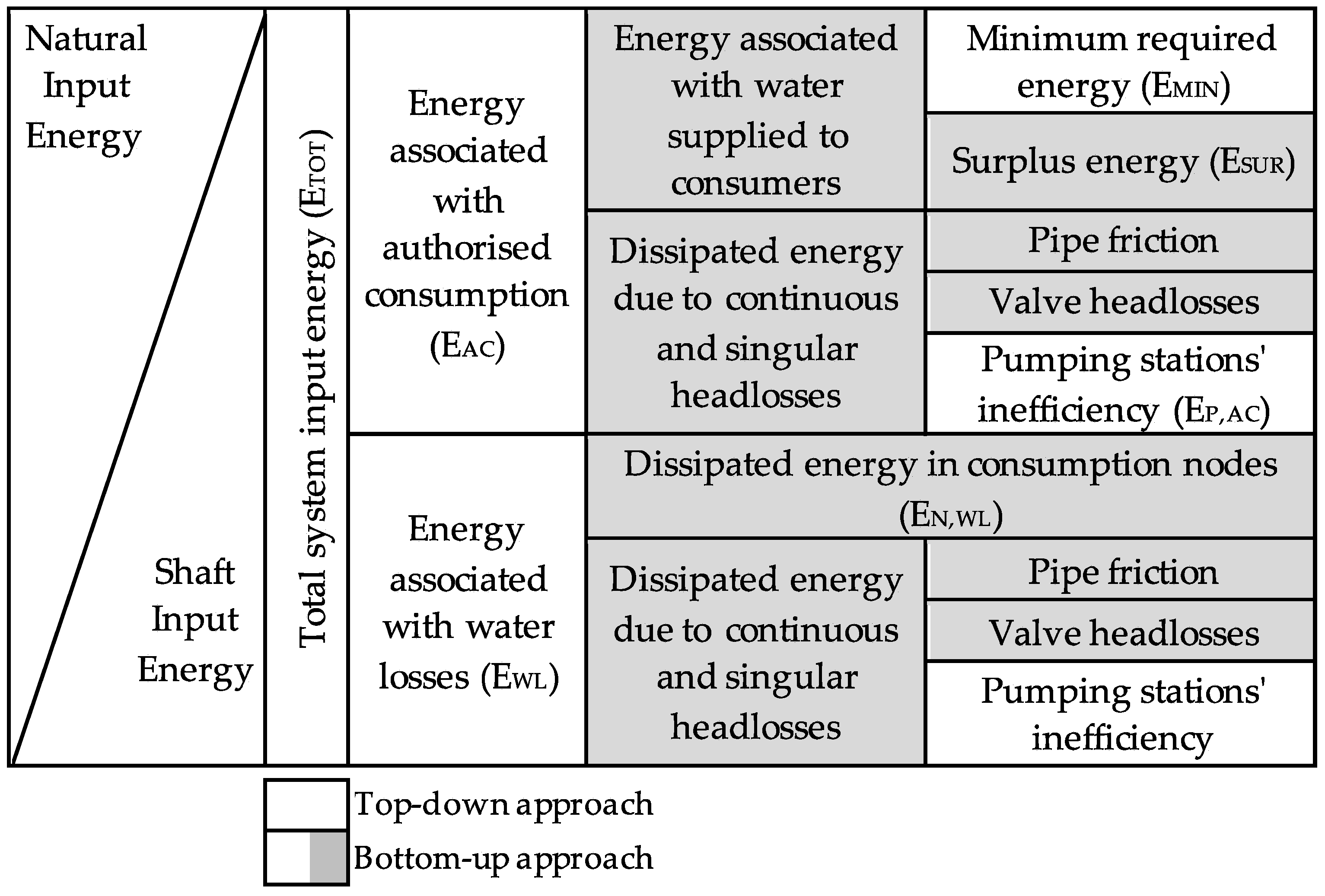
The WEB proposed by [14] is depicted in Figure 1 for systems without energy recovery. System input energy is calculated as the sum of natural and shaft input energy. Natural input energy refers to the potential energy supplied by reservoirs, storage tanks, or pressurized delivery points at the entrance of the system. Shaft input energy refers to the energy supplied by all pumping stations. System input energy is, then, divided in two parts: energy associated with authorized consumption (EAC) and associated with water losses (EWL). EAC includes the energy associated with the water supplied to consumers and the dissipated energy due to headlosses in the system and inefficiencies in pumps. The energy associated with water delivered to consumers includes the minimum required energy and surplus energy. The first is the theoretical minimum energy needed in the case of a frictionless system. Since the supplied pressure can be higher than the minimum required pressure, there is surplus energy in the system. Continuous headlosses associated with pipe friction, singular headlosses associated to valves, and pump inefficiencies are considered in the WEB. EWL includes the energy associated with water losses (lost in transport, valves, pumps, and leaks). For modelling purposes, water losses are typically attributed to consumption nodes and minimum pressure for the calculation of minimum energy is considered uniform for each system (typically, 15 or 25 m in Portugal). Energy balance components are calculated in relation to a reference value adopted as the minimum elevation point of the system. The WEB can be assessed using top-down or bottom-up approaches. The former begins with the calculation of the main energy balance components (see components without shade in Figure 1), while the latter goes from the specific components to the general ones. The main differences of each approach are given in the following subsections.
Comparison between systems is achieved through the calculation of energy performance indicators. Table 1 shows the calculation of energy performance indicator E3 and its partition in the main energy inefficiencies. E3 represents a ratio of the theoretic energy in excess that is supplied to the system in comparison to the minimum energy required. E3 can be assessed in terms of dissipated energy in pumps, E3 (pumps). Energy inefficiencies associated with water losses are given by assessing E3 (losses). Energy in excess due to network operation and layout inefficiencies are given by assessing E3 (network). This indicator E3 includes the surplus energy and dissipated energy in pipes and valves due to consumption (components that are only calculated in the bottom-up approach) but can be directly calculated in the top-down approach, as showed in Table 1. This allows an efficient diagnosis of the main network inefficiencies, even in the top-down approach.
2.1. Top-Down Approach
The top-down approach (or simplified assessment [14]) requires minimum data (i.e., no hydraulic model is needed) and provides a global overview of the main components of energy consumption in the system: natural input energy, shaft input energy, energy associated with consumption and water losses, and minimum energy and pump inefficiencies (related to consumption and losses). Required data include: inlet water volumes and hydraulic heads at delivery points, storage tanks and pumping stations, and electric energy consumption in each pumping station for a preliminary calculation of the pumping station’s efficiency. The system should also be divided in homogeneous areas with similar pressure requirements where authorized consumption and the center of mass of consumption is known. The pressure value depends on the characteristics of the area (e.g., size, type of buildings). Results obtained for minimum required node pressure typically ranges between 1.5 and 3.0 bar (in Portugal). Minimum energy in the top-down approach is calculated as follows:
where γ is water specific weight (N/m3); is the annual authorised consumption (m3); is the center of mass of consumption; is the minimum pressure required (m) in the analysis area a; z0 is the reference elevation (m); and α is the conversion factor from Ws to kWh, 1/(1000 × 3600) = 2.78 × 10⁻⁷.
Finally, the percentage of water losses and authorized consumption in the system should be collected from the water balances. The main assumption for this assessment (referred, herein, as reference method M0) is that the energy associated with water losses is proportional to the water loss percentage.
2.2. Bottom-Up Approach
The bottom-up approach (or complete assessment [14]) requires a calibrated hydraulic model of the network and provides a detailed assessment of energy consumption in each component of the balance. This approach requires a calibrated and reliable hydraulic model of the network [14]. Two methods can be used to implement this assessment. The first method (M1) assumes that water losses are proportional to node demand and involves the calculation of two simulations (with and without water losses). The simulation of water losses is achieved by dividing the original demand multiplier by the percentage of authorized consumption. The second method assumes (M2) that water losses (real) are proportional to pressure and to the length of pipes confluent to each node, and so, requires the redistribution of water losses accordingly. This is an iterative procedure that requires the calibration of emitter coefficients in network nodes as well as the setting of an emitter exponent, as explained by [16].
To better understand the differences between M1 and M2, the calculation of minimum energy, surplus energy, and dissipated energy in consumption nodes is reviewed. Minimum required energy is calculated using Equation (2) for both methods:
where d refers to the simulation without water losses (i.e., by using the original demand multiplier of the model), being given by the ratio between authorized consumption (AC) and the total input volume including water losses (TIV); is the node consumption (m3/s) at time t; is the node elevation (m); is the minimum required pressure at node n (m); z0 is the reference elevation (m); is the time duration; nn is the number of nodes; and nt is the number of time steps (usually each time step has a 15 min duration).
The supplied pressure can be higher than , creating surplus energy in the system. Equation (3) shows the calculation of surplus energy for both methods:
where is the node head (m) at time t.
Dissipated energy in consumption nodes is calculated as follows, for M1 and M2, respectively:
where d = 1 refers to the simulation including water losses (i.e., by dividing the original demand multiplier by the percentage of authorized consumption) and is the leak flow at time t.
3. Case Studies
Twenty real networks from Portuguese water distribution systems have been analyzed in order to test the stated hypothesis (i.e., percentage of dissipated energy associated with water losses is equal to the percentage of water losses) and to calculate the WEB components. The main characteristics of the analyzed systems are summarized in Table 3. The median values for each characteristic are also presented. Network length varied between 4 and 114 km and elevation difference (Δz) varied between 6 and 96 m. Average diameter weighted by pipe length ranged between 60 and 150 mm. Average pressure weighted by demand ranged between 16 and 55 m, average velocity weighted by pipe length ranged between 0.02 and 0.2 ms−1, and average headlosses weighted by pipe length ranged between 0.05 and 1.6 mkm−1. The Hazen–Williams headloss formula was adopted since the flow regime is typically turbulent in water distribution systems [17]. Plastic (C = 135–145) was the predominant pipe material, although some networks still had some asbestos cement pipes (C = 90). Water losses ranged between 3% and 50% and most systems were gravity-fed.
The assessment of energy efficiency in gravity-fed systems is relevant, despite having no costs associated with energy consumption for two main reasons:
- The assessment of surplus energy helps evaluating excessive pressures in the system and may even indicate opportunities for water loss reduction and for energy recovery (especially in transmission systems).
- It is highly probable to have energy consumption (associated with water treatment and transport) that might be reduced at the systems upstream. For instance, if water losses are reduced through the reduction of energy associated with water losses, less energy needs to be treated and transported.
Water losses above 30% occur due to a variety of reasons: ageing networks, illegal connections, and absence of reading meters and procedures. Carrying out water balances to understand the impact of real and apparent losses is the first step to define improvement solutions in these systems. On the other hand, systems ID13 and ID14 corresponded to a touristic area fully equipped with a telemetry system and a well-maintained infrastructure with low water losses.
Regarding water sources, two systems (ID1 and ID6) had their water source in groundwater wells with shaft energy representing 100% of total input energy. In these systems, every additional unit of water (increased consumption and/or losses) required more energy since the groundwater tables go down when more water is pumped up. The remaining systems were distribution networks, with the water source in network delivery points that supply water to storage tanks. Three systems had shaft energy ranging between 11% and 77% with pumping stations that ensure water supply in high elevation points (ID3, ID8, and ID9).
Systems ID3, ID4, and ID5 represent the same system, but for different operating configurations (with pump, with layout change and pressure-reducing valve, and with layout change, respectively). System ID 13 and ID14 also represent the same system, for winter and summer scenarios, respectively.
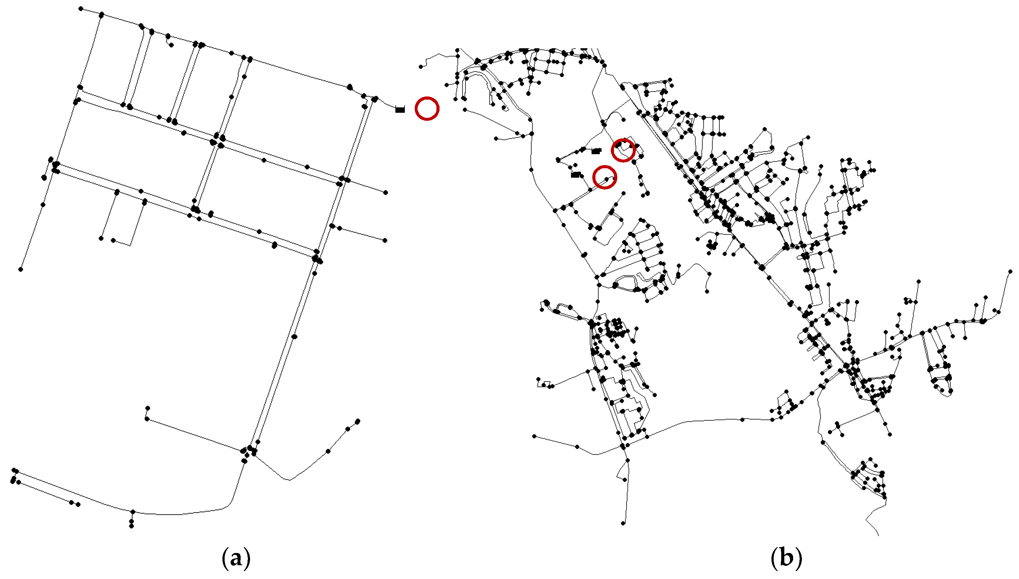
Analyzed networks have different forms and complexities. Figure 2 shows two examples of network models. Figure 2a represents gravity system ID16 with 219 nodes and 5 km. Figure 2b represents rising system ID6, a more complex model with 2042 nodes and 70 km.
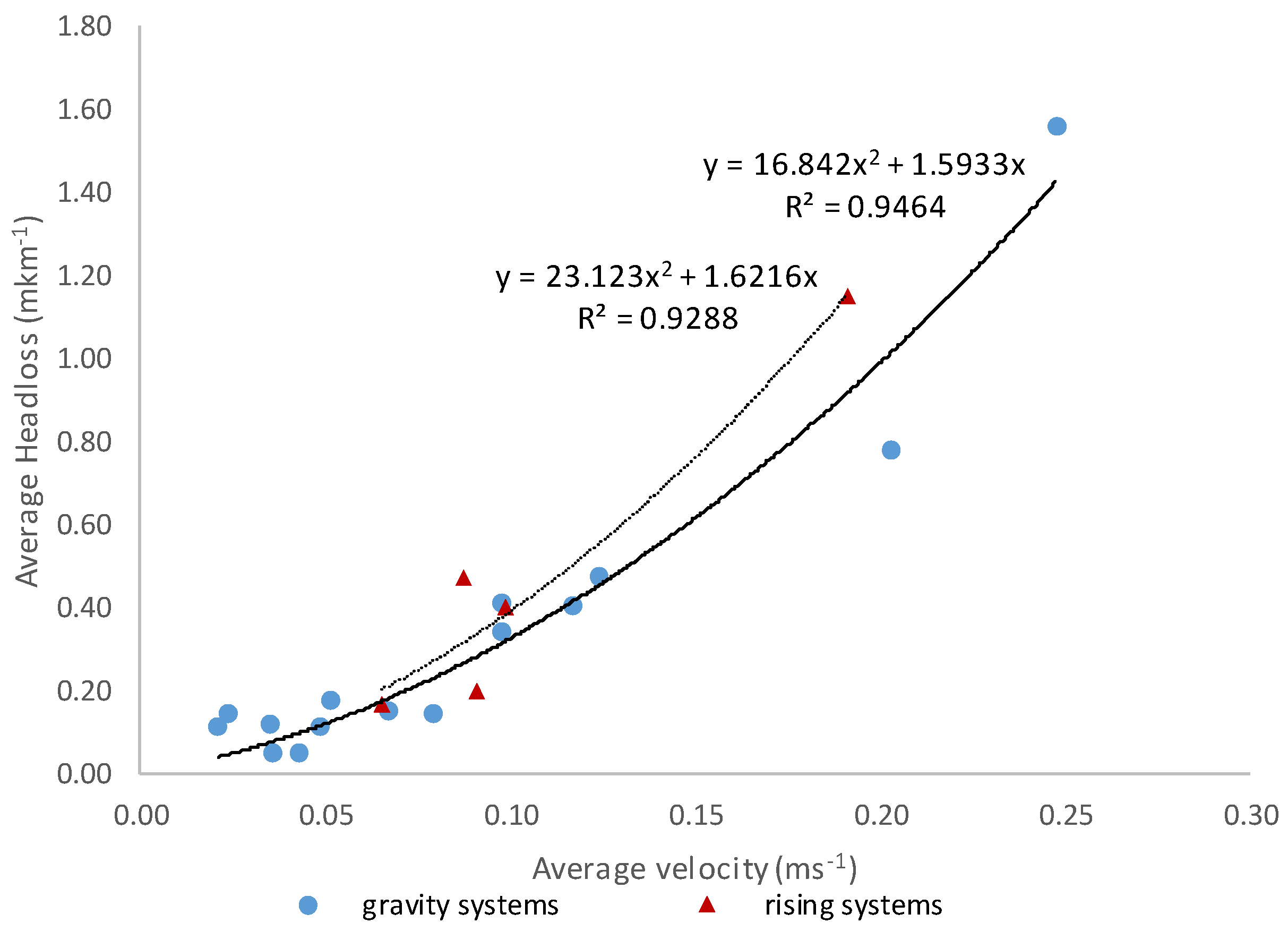
Figure 3 shows the results of average headlosses as a function of average flow velocity for analyzed gravity and rising systems. Average headlosses were below 0.60 mkm−1, while the average velocity for most of the systems was below 0.15 ms−1—much below the national legislation values for distribution systems (between 0.3 and 1 ms−1). Low velocities in real distribution systems have already been verified by [18].
In Portugal, overdesigned distribution systems are common due to firefighting requirements and the overestimation of population and water demand. Low velocities potentiate problems with water quality and sediment deposition [19]. A second-degree polynomial trendline has been fitted for gravity and rising systems. Most of the models are overdesigned, as they are located in the lower part of the curve (i.e., velocities < 0.10 ms−1), meaning that by adding water losses, flow and velocity will increase, with a slight impact on headlosses. The trendline for rising systems is more inclined, meaning that systems with shaft energy will have higher changes in headloss as a response to changes in velocity, and therefore, to changes in flow.
4. Results
4.1. Comparison of Top-Down and Bottom-Up Approaches
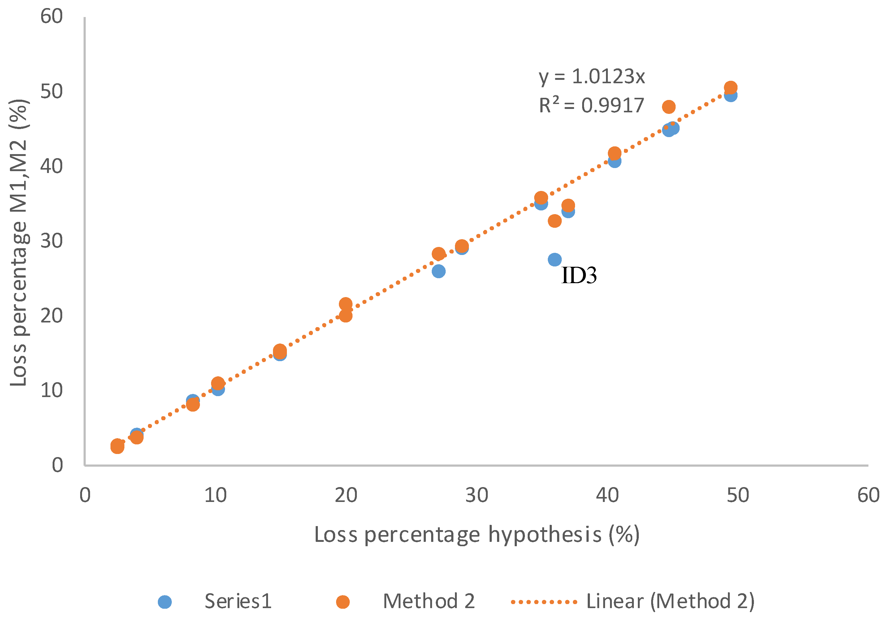
Figure 4 presents the results of energy associated with water losses (EWL) in percentage calculated for the bottom-up approach using M1 and M2 against the loss percentage hypothesis M0 given by the loss percentage from water balances in the top-down approach. For most tested models, results are very similar for M1 and M2, meaning that assumption M0 is valid and, therefore, the top-down approach is valid. A linear trendline has been fitted for method M2. Calibrated emitter coefficients for M2 range between 3.7 × 10⁻⁷ and 8.8 × 10⁻⁵ (L/s/m/mβ).
The main differences between the results obtained for M0 and M1 have been observed for systems with pumping stations. The hydraulic head provided by these systems is defined by pump characteristics curves Q-H, described by quadratic curves in which each unit of flow increase (e.g., due to water losses) means a quadratic decrease in the supplied head. This means that systems with shaft energy are more responsive to changes is flow and, therefore, high water losses originate a considerable decrease in the node pressure, reducing the EWL for M1. Systems with variable-speed pumps are probably less responsive to changes is flow, since pressure can be more stable to network flow variation. In general, gravity-fed systems face fewer significant changes in the hydraulic supplied head when water losses are added, and consequently, similar results for EWL were obtained for M0 and M1. Results for M0 and M2 are very similar, regardless of shaft energy. Despite water losses affecting the pump curves in the same way as in M1, water losses are higher in nodes with higher pressure, which results in EWL values close to the ones obtained by M0.
System ID3 (identified in Figure 4) is the one with the highest error between the hypothesis and the calculated EWL (M0 = 36%, M1 = 28%, M2 = 33%). The differences between the three methods are primarily attributed to the fact that friction losses do not vary linearly with velocity (and flow), as illustrated in Figure 2. System ID3 has an average velocity of 0.09 m/s. When water losses are proportionally added to demand, this velocity increases proportionally to 0.14 m/s, and the system is more reactive to changes in flow. Despite this fact, the maximum difference between M0 and M1 is still low (8%) compared to the uncertainties associated with the required data (elevations, water volumes), typically ranging between 6% and 20% according to a survey carried in the utilities.
Methods M1 and M2 give different results due to the calculation method. Water losses in method M1 are distributed proportionally to water demand. In method M2, the losses distribution is higher in the nodes with higher pressure and in the nodes associated with long pipes.
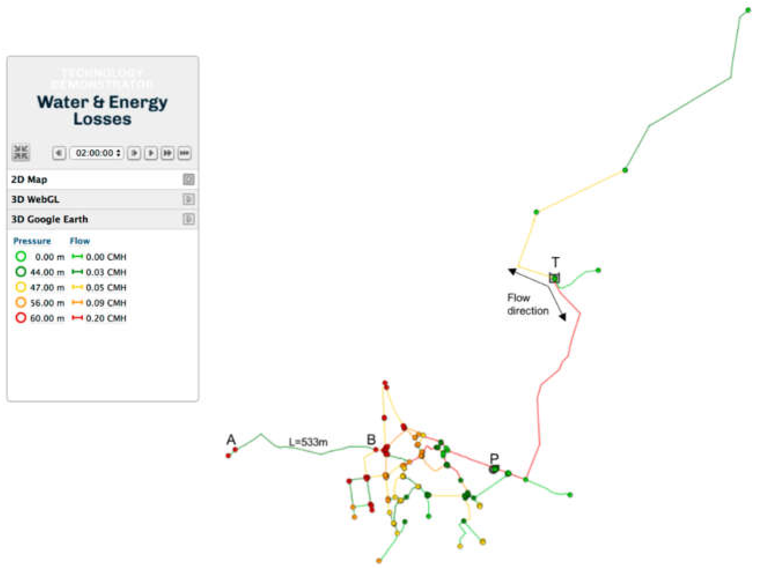
Figure 5 shows the network model for system ID3 and the simulation results for pressure and flow between 1:00 and 2:00 a.m., the minimum night consumption period. Water is supplied by a storage tank in two directions. Downstream of the tank, there is a pump that supplies water to high elevation nodes, creating excessive pressure in some areas. As depicted, the pipe that connects nodes A and B (L = 533 m) has high pressure levels (above 60 m). According to the calculations, these nodes are responsible for 17% of the water losses distribution in M2. This value is much higher than for M1, where nodes A and B only account for 6% of the water losses.
The total simulated water losses are the same, only their spatial distribution varies along the system. Since energy is influenced by pressure and flow, and for M1 higher losses (higher flows) occur in nodes with lower pressures (as opposite to M2), EWL will be lower for method M1. If the majority of water losses are real and, therefore, pressure-dependent [20], then method M2 is more accurate and recommendable to estimate this component. Since method M1 has provided good results for most of the cases, this method can always be implemented, except for systems with shaft energy and high real losses with percentages above 30%. In this latter case, method M2 is recommended to estimate water losses and to carry out the WEB.
4.2. Water-Energy Balance Components and Performance Indicators
No significant differences between M1 and M2 were found for the energy balance components.
Figure 6 presents the median values for gravity-fed and rising systems as well as the 5th and 95th percentile for the WEB components using M2. The WEB has been simplified in the subcomponents of EWL since the values were not significant.
For the 20 network models analyzed, 15 are gravity-fed (G) and 5 are rising (R). The following paragraphs refer to the median values obtained for each WEB component for the two system types. In gravity-fed systems, 80% of the supplied energy is associated with authorized consumption and 20% with water losses. In rising systems, water losses are higher, representing 28% of total input energy.
From the energy associated with consumption, the energy associated with water supplied to consumers represents 74% in gravity-systems and is 11% lower in rising systems. Minimum required energy represents 40% in both system types. Surplus energy in gravity systems is 28% and 16% in rising systems. Dissipated energy due to continuous and singular headlosses represents only 1% in gravity systems, while in rising systems it is 26% due to the dissipated energy in pumping stations. Valve headlosses in pressure-reducing valves can represent up to 15% in some systems.
From the energy associated with water losses, the majority is in consumption nodes and accounts for 19% and 13% of total input energy for gravity and rising systems, respectively. The energy dissipated in continuous and singular headlosses due to water losses is low.
In summary and in median terms, the major inefficiencies in gravity-fed systems are due to surplus energy (28%) and losses in consumption nodes (19%). Major inefficiencies in rising systems are due to surplus energy (16%), dissipated energy in pumps (16%), and node water losses (13%). However, looking at the ranges obtained, each of the referred WEB components (surplus energy, pump inefficiencies, and water losses) can reach 40% of total input energy. Less significant components are pipe friction and valve headlosses, each reaching up to 15% of total input energy.
Figure 7a shows the main results from the top-down approach. Performance indicator E3 evaluates the ratio of total energy in excess [14]. E3 ranges between 0.5 and 5.5, which means that energy in excess can represent 5.5 times the minimum required energy. E3 can be divided into three main components: network (surplus energy and continuous and singular headlosses related to water consumption), losses (includes all components of EWL), and pump (pump inefficiencies related to water consumption). On average, 53% of inefficiencies are network-related, 39% are losses-related, and 8% are pump-related. Figure 7b presents results for the bottom-up approach, representing energy inefficiencies sorted by decreasing value of E3 and grouped as follows: surplus energy, continuous and singular headlosses (includes pipe friction and valve headlosses associated with water consumption), water losses (includes node water losses, pipe friction, valve headlosses and pump inefficiencies associated with water losses), and pumping station inefficiencies associated with consumption. Systems are sorted by descending order of E3—the ratio of energy in excess.
Surplus energy is the most relevant inefficiency, except for systems ID3 and ID1, where water losses and pump inefficiencies are more critical. Surplus energy can be reduced through changes in layout or operation modes and through pressure management. Systems ID4, ID1, and ID15 have important headlosses that are associated with valves (ID4 and ID15) and high seasonality in consumption flows (ID1). High valve headlosses might indicate potential for network layout improvements. Water losses are the second highest inefficiency for most systems and can be reduced through a rigorous assessment of the water balance and associated performance indicators [21]. System ID3 is the most inefficient since energy in excess represents 5.5 times the minimum energy: 54% of this inefficiency is associated with pumps, 43% to water losses, and 3% to network layout. As previously referred, ID4 and ID5 refer to the same system with different operating conditions where the pump is deactivated. ID5 has an E3 = 1.2, which is a considerable improvement compared to the initial value, though some improvements in terms of surplus energy can still be achieved. Systems ID13 and ID14 are the ones with better overall energy efficiency, since energy in excess represents less than minimum required energy. Based on the results obtained for these models, reference values for E3 can be established for ∆z < 100 m, as follows:
- [0,1]: good service level with total energy inefficiencies below 40%.
- [1,2]: median service level with total energy inefficiencies below 65%.
- [2,+∞]: unsatisfactory service level with total energy inefficiencies above 65%.
The importance of establishing a limit for ∆z lies in the fact that E3 tends to 0 for high elevation differences between the reference elevation and the supply or consumption elevation. Results also show that in most cases, a top-down approach is enough to diagnose the main energy inefficiencies and test improvement solutions. For instance, looking at systems ID20 and ID4, both have similar values of E3, but ID20 has a high water loss percentage (E3 loss = 56% in Table 1), while ID4 has 80% of its energy inefficiencies in the network (E3 network = 80% in Table 1). This is confirmed in Figure 7, where ID20 shows high EWL and ID4 has high headlosses. Therefore, bottom-up assessments can be important for systems with E3 > 2 and low percentage of water losses (e.g., below 15%) and low pump inefficiencies (e.g., Ph5 > 0.4 kWh/(m3∙100 m)). In the case of high water losses, the water balance can be assessed to check whether real or apparent losses are the most significant. In the case of high pump inefficiencies, the Ph5 indicator can indicate pump efficiency, and if the pump is really needed and no alternative layout is feasible, energy audits can be carried out to assess how to improve pump efficiency.
5. Discussion
The hypothesis that energy associated with water losses (EWL) is proportional to the water loss percentage given by water balances is valid, as corroborated by the two methods used in the bottom-up approach results. The first method (M1) assumes losses proportional to demand in network nodes and is implemented by running two simulations and setting a demand multiplier according to the water loss percentage. The second (M2) assumes a distribution of water losses that is pressure-dependent and is implemented by calibrating emitter exponents in an iterative procedure. No significant differences between methods M1 and M2 have been found, except for one model with losses >36% and a significant average pressure of 47 m. For comparison purposes, apparent losses have not been considered in this study (all water losses have been assessed as real losses in the application of method M2). However, method M1 might be more suited when apparent losses are predominant and method M2 when real losses are predominant or when water losses are higher than 30% and there is shaft energy.
The 20 networks where the methodology was applied are mostly distribution systems with different sizes and topologies. In the studied systems, the most important energy inefficiencies are associated with surplus energy and water losses, reaching up to 40% and 48% of total input energy, respectively. A fixed minimum pressure for every node is assumed, which might be influencing the surplus energy results in cases where distribution systems are not homogeneous in terms of occupancy (e.g., skyscrapers with houses in the same elevation curve). Pump inefficiencies are also relevant, but are not usually the most significant component, reaching 10%–25%. This highlights the importance of carrying out a system analysis rather than the traditional equipment-centered analysis that only allows comparing equipment efficiencies, disregarding other inefficiencies types [22].
The definition of surplus energy as a system inefficiency is also a novel contribution compared to previous works [10] and allows for understanding how much energy in excess is delivered to consumers compared with the minimum required energy. Reducing surplus energy to zero is theoretically impossible since there are always friction losses in WSS. Nevertheless, some systems may achieve important reductions, for instance, by reducing the service pressure.
These learnings can be transferred to any WWS in the world, since the analyzed case studies are significantly different from each other and the methodology is not case dependent. The WEB component values may, however, be different in other WSS. For instance, transmission systems may behave differently and should also be analyzed in terms of the most significant WEB components.
Reference values for energy efficiency indicator E3, which represents the ratio of total energy in excess, have been provided for systems with ∆z < 100 m. E3 < 1 represents a good service level, whereas E3 > 2 represents an unsatisfactory service level.
Regarding network models, there are still important difficulties, namely, pump curves are sometimes modelled with a single point, or with the fabricant curve, not reflecting the real operating conditions, and utilities are unaware of the controls behind variable speed pumps. These difficulties end up limiting the analysis of models with shaft energy.
6. Conclusions
This paper presents a top-down and a bottom-up approach for carrying out water-energy balances (WEB) in water supply systems. The top-down approach is easy to implement, requires minimum data, and provides an effective diagnosis of energy inefficiencies. This approach lays its foundation in the hypothesis that energy due to water losses is proportional to water loss percentages. This may not always be true since the flow regime may lead to headlosses varying in a second-order degree with flow. The hypothesis has been validated for 20 real network models using two different methods of water losses distribution throughout the network nodes. Energy inefficiencies can be efficiently tracked in the top-down approach using the energy performance indicator E3 and its subcomponents (pumps, losses, and network). The bottom-up approach requires a calibrated hydraulic model of the network and provides a detailed analysis of dissipated energy in pipes, valves, and surplus energy. This is essential to compare improvement solutions associated with changes in operation and layout and network rehabilitation. Median results show that minimum energy accounts for nearly 40% of total input energy, dissipated energy due to water losses represents 20%–30% (for gravity and rising systems, respectively), surplus energy represents 16%–28% (for rising and gravity systems, respectively), and dissipated energy in pumps represents 16%. Continuous headlosses only represent 1%–3% of total energy.
Future developments include the release of a computational framework that allows the automatic calculation of the bottom-up assessment.
Author Contributions
The conceptual idea of this paper was brought up by Helena Alegre. Data analysis and investigation was carried out by Aisha Mamade. The Writing-Review & Editing was accomplished by Aisha Mamade, Dália Loureiro, Dídia Covas. Dídia Covas was also responsible for funding acquisition.
Funding
This research was funded by Fundação para a Ciência e a Tecnologia (FCT), PhD Grant PD/BD/105968/2014., by the European Commission’s FP7 financial support for TRUST project (Grant Agreement number 265122) and by the EC LIFE Programme Smart Water Supply System project (LIFE14 ENV/PT/000508).
Acknowledgments
The authors would like to thank the 17 water utilities that participated in iPerdas project (www.iPerdas.org). A special thanks for Paulo Praça, from CM Barreiro.
Conflicts of Interest
The authors declare no conflict of interest.
References
- Barry, J.A. Watergy: Energy and Water Efficiency in Municipal Water Supply and Wastewater Treatment. Cost-Effective Savings of Water and Energy; Alliance to Save Energy: Washington, DC, USA, 2007; Available online: http//watergy.org/resources/publications/watergy.pdf (accessed on 19 March 2018).
- Mabhaudhi, T.; Mpandeli, S.; Madhlopa, A.; Modi, A.T.; Backeberg, G.; Nhamo, L. Southern Africa’s water-energy nexus: Towards regional integration and development. Water 2016, 8, 235. [Google Scholar] [CrossRef]
- Lenzi, C.; Bragalli, C.; Bolognesi, A.; Artina, S. From energy balance to energy efficiency indicators including water losses. Water Sci. Technol. Water Supply 2013, 13, 889–895. [Google Scholar] [CrossRef]
- Yoon, H.; Sauri, D.; Amorós, A.R. Shifting Scarcities? The Energy Intensity of Water Supply Alternatives in the Mass Tourist Resort of Benidorm, Spain. Sustainability 2018, 10, 824. [Google Scholar] [CrossRef]
- Suárez, F.; Muñoz, J.F.; Fernández, B.; Dorsaz, J.-M.; Hunter, C.K.; Karavitis, C.A.; Gironás, J. Integrated Water Resource Management and Energy Requirements for Water Supply in the Copiapó River Basin, Chile. Water 2014, 6, 2590–2613. [Google Scholar] [CrossRef]
- Aubuchon, C.P.; Roberson, J.A. Evaluating the embedded energy in real water loss. J. Am. Water Works Assoc. 2014, 106, 129–138. [Google Scholar] [CrossRef]
- Vilanova, M.R.N.; Balestieri, J.A.P. Exploring the water-energy nexus in Brazil: The electricity use for water supply. Energy 2015, 85, 415–432. [Google Scholar] [CrossRef]
- ERSAR. Annual Report on Water and Waste Services in Portugal; ERSAR (Portuguese Water and Waste Regulator): Lisbon, Portugal, 2017. [Google Scholar]
- Copeland, C. Energy-Water Nexus: The Water Sector’s Energy Use; Congressional Research Service: Washington, DC, USA, 2014.
- Cabrera, E.; Pardo, M.A.; Cobacho, R.; Cabrera, E., Jr. Energy audit of water networks. J. Water Resour. Plan. Manag. 2010, 136, 669–677. [Google Scholar] [CrossRef]
- Walski, T. Energy Balance for a Water Distribution System. In World Environmental and Water Resources Congress 2016; ASCE: Reston, VA, USA, 2016; pp. 426–435. [Google Scholar]
- Carriço, N.; Covas, D.; Alegre, H.; do Céu Almeida, M. How to assess the effectiveness of energy management processes in water supply systems. J. Water Supply Res. Technol. 2014, 63, 342–349. [Google Scholar] [CrossRef]
- Sarbu, I. A Study of Energy Optimisation of Urban Water Distribution Systems Using Potential Elements. Water 2016, 8, 593. [Google Scholar] [CrossRef]
- Mamade, A.; Loureiro, D.; Alegre, H.; Covas, D.D. A comprehensive and well tested energy balance for water supply systems. Urban Water J. 2017, 14, 853–861. [Google Scholar] [CrossRef]
- Loureiro, D.; Mamade, A.; Ribeiro, R.; Vieira, P.; Alegre, H.; Coelho, S.T. Implementing water-energy loss management in water supply systems through a collaborative project. In Proceedings of the IWA Water Loss Conference, Vienna, Austria, 31 March–2 April 2014. [Google Scholar]
- Covas, D.I.C.; Jacob, A.C.; Ramos, H.M.; Jacob, A.C.; Ramos, H.M. Water losses’ assessment in an urban water network. Water Pract. Technol. 2008, 3, 1–9. [Google Scholar] [CrossRef]
- Walski, T.M.; Chase, D.V.; Savic, D.A. Water Distribution Modeling; Haestad Press: Waterbury, CT, USA, 2001; p. 72. [Google Scholar]
- Vidigal, P.M.; Covas, D.I.C.; Loureiro, D.; Coelho, S.T.; Alegre, H. Extensive analysis of hydraulic parameters in a large set of water distrubution systems. In Proceedings of the Tenth International Conference on Computing and Control for the Water Industry, CCWI 2009, Sheffield, UK, 1–3 September 2009. [Google Scholar]
- Poças, A. Discolouration Loose Deposits in Distribution Systems: Composition, Behaviour and Practical Aspects. Ph.D. Thesis, Delft University of Technology, Delft, The Netherlands, 2014. [Google Scholar]
- Lambert, A. What Do We Know About Pressure: Leakage Relationships In Distribution Systems? In Proceedings of the System Approach to Leakage Control and Water Distribution Systems Management: IWA International Specialised Conference, Brno, Czech, 16–18 May 2001; pp. 1–8. [Google Scholar]
- Farley, M.; Trow, S. Losses in Water Distribution Networks. A Practitioner’s Guide to Assessment, Monitoring and Control; IWA Publishing: London, UK, 2003. [Google Scholar]
- HDR Engineering. Handbook of Energy Auditing of Water Systems; HDR Engineering: Omaha, NE, USA, 2011; p. 109. [Google Scholar]
Figure 1.
Water-energy balance (WEB) for systems without energy recovery (adapted from [14]).
Figure 1.
Water-energy balance (WEB) for systems without energy recovery (adapted from [14]).

Figure 2.
Examples of tested network models (a) gravity with water source in tank, ID16 (b) rising with water source in wells, ID6.
Figure 2.
Examples of tested network models (a) gravity with water source in tank, ID16 (b) rising with water source in wells, ID6.

Figure 3.
Average headloss and velocity for the tested network models.

Figure 4.
Loss percentage for Method 1 and Method 2 compared to loss percentage hypothesis.

Figure 5.
Simulation results for System ID3 (T = Tank, P = Pump).

Figure 6.
Median values for gravity-fed (G) and rising (R) systems and ranges (5th–95th percentile) for WEB components using M2.
Figure 6.
Median values for gravity-fed (G) and rising (R) systems and ranges (5th–95th percentile) for WEB components using M2.

Figure 7.
(a) E3 (ratio of energy in excess) split by inefficiencies due to network, losses, and pumps (top-down approach) and (b) components of energy inefficiencies given by the bottom-up approach.
Figure 7.
(a) E3 (ratio of energy in excess) split by inefficiencies due to network, losses, and pumps (top-down approach) and (b) components of energy inefficiencies given by the bottom-up approach.


Table 1.
Energy performance indicator E3 and its partition in main inefficiencies (adapted from [14]).
Table 1.
Energy performance indicator E3 and its partition in main inefficiencies (adapted from [14]).
| E3—Ratio of the total energy in excess (-) | |
| E3 (pumps)—Ratio of the energy in excess due to dissipated energy in pumps | |
| E3 (losses)—Ratio of the energy in excess due to water losses | |
| E3 (network)—Ratio of the energy in excess due to network operation and layout |
Table 2.
Summary of required data, main assumptions, and EWL assessment for top-down and bottom-up approaches.
Table 2.
Summary of required data, main assumptions, and EWL assessment for top-down and bottom-up approaches.
| Approach | Abbreviation | Required Data | Assumptions | EWL Assessment |
|---|---|---|---|---|
| Top-down | M0 |
| Energy associated with water losses is proportional to water loss percentage from water balances (hypothesis). | % Water losses |
| Bottom-up | M1 |
| Water losses are distributed proportionally to flow. | Demand multiplier, difference between simulation with and without losses |
| M2 | Water losses are distributed proportionally to pressure and to pipe length. | Calibrated emitter coefficients, emitter exponent (set as 1.18) |
Table 3.
Case study characterization.
| ID | Length | ∆z | Water Loss | Shaft Energy | Average Diameter | Average Pressure | Average Velocity | Average Headloss |
|---|---|---|---|---|---|---|---|---|
| (km) | (m) | (%) | (%) | (mm) | (m) | (ms−1) | (mkm−1) | |
| 1 | 114.6 | 66.2 | 37.1 | 99.3 | 106 | 17 | 0.19 | 1.2 |
| 2 | 58.6 | 28.5 | 35.0 | 0.0 | 99 | 35 | 0.05 | 0.2 |
| 3 | 9.6 | 47.5 | 36.0 | 76.5 | 64 | 44 | 0.10 | 0.4 |
| 4 | 9.1 | 47.5 | 15.0 | 0.0 | 64 | 31 | 0.05 | 0.1 |
| 5 | 9.1 | 47.5 | 15.0 | 0.0 | 60 | 47 | 0.09 | 0.5 |
| 6 | 69.5 | 50.7 | 4.0 | 99.9 | 114 | 43 | 0.10 | 0.4 |
| 7 | 34.8 | 32.7 | 10.2 | 0.0 | 100 | 34 | 0.10 | 0.3 |
| 8 | 57.3 | 37.9 | 27.2 | 10.9 | 124 | 31 | 0.09 | 0.2 |
| 9 | 72.5 | 55.5 | 8.4 | 52.0 | 107 | 37 | 0.07 | 0.2 |
| 10 | 51.2 | 74.2 | 44.8 | 0.0 | 87 | 45 | 0.02 | 0.1 |
| 11 | 9.8 | 6.7 | 40.7 | 0.0 | 85 | 23 | 0.02 | 0.1 |
| 12 | 4.8 | 57.9 | 49.6 | 0.0 | 106 | 46 | 0.04 | 0.1 |
| 13 | 76.5 | 40.2 | 2.5 | 0.0 | 135 | 37 | 0.04 | 0.1 |
| 14 | 76.5 | 40.2 | 2.5 | 0.0 | 135 | 35 | 0.12 | 0.5 |
| 15 | 22.3 | 96.0 | 29.0 | 0.0 | 117 | 41 | 0.12 | 0.4 |
| 16 | 5.2 | 26.7 | 20.0 | 0.0 | 109 | 30 | 0.25 | 1.6 |
| 17 | 4.4 | 30.0 | 20.0 | 0.0 | 112 | 44 | 0.08 | 0.1 |
| 18 | 10.2 | 48.7 | 20.0 | 0.0 | 149 | 45 | 0.07 | 0.2 |
| 19 | 16.9 | 41.3 | 20.0 | 0.0 | 131 | 38 | 0.04 | 0.1 |
| 20 | 9.3 | 41.4 | 45.1 | 0.0 | 151 | 55 | 0.20 | 0.8 |
| Median | 19.6 | 44.5 | 20.0 | 0.0 | 108 | 38 | 0.08 | 0.19 |
© 2018 by the authors. Licensee MDPI, Basel, Switzerland. This article is an open access article distributed under the terms and conditions of the Creative Commons Attribution (CC BY) license (http://creativecommons.org/licenses/by/4.0/).
Share and Cite
MDPI and ACS Style
Mamade, A.; Loureiro, D.; Alegre, H.; Covas, D. Top-Down and Bottom-Up Approaches for Water-Energy Balance in Portuguese Supply Systems. Water 2018, 10, 577. https://doi.org/10.3390/w10050577
AMA Style
Mamade A, Loureiro D, Alegre H, Covas D. Top-Down and Bottom-Up Approaches for Water-Energy Balance in Portuguese Supply Systems. Water. 2018; 10(5):577. https://doi.org/10.3390/w10050577
Chicago/Turabian StyleMamade, Aisha, Dália Loureiro, Helena Alegre, and Dídia Covas. 2018. "Top-Down and Bottom-Up Approaches for Water-Energy Balance in Portuguese Supply Systems" Water 10, no. 5: 577. https://doi.org/10.3390/w10050577
Note that from the first issue of 2016, this journal uses article numbers instead of page numbers. See further details here.