Quantitative Assessment of Flow Regime Alteration Using a Revised Range of Variability Methods


1
State Key Laboratory of Simulation and Regulation of Water Cycle in River Basin, China Institute of Water Resources and Hydropower Research, Beijing 100038, China
2
Department of Water Environment, China Institute of Water Resources and Hydropower Research, Beijing 100038, China
3
National Institute of Water and Atmospheric Research Ltd., Christchurch 8440, New Zealand
*
Author to whom correspondence should be addressed.
Water 2018, 10(5), 597; https://doi.org/10.3390/w10050597
Submission received: 19 March 2018
/
Revised: 27 April 2018
/
Accepted: 28 April 2018
/
Published: 4 May 2018
(This article belongs to the Section Hydrology)
Abstract
:The Ecological Limits of Hydrologic Alteration (ELOHA) framework, which can be used to determine and implement environmental flows at regional scales, requires accurate flow regime alteration assessment. The widely used range of variability approach (RVA) evaluates flow regime alteration by comparing the distribution of 32 Indicators of Hydrologic Alteration (IHA). However, the traditional RVA method is not comprehensive, because it neglects both the human-induced inner characteristics of one hydrological year (ICOHY) and the positional information of 32 IHA, which are the main factors behind ecosystem alteration. To address these limitations, we propose a revised RVA method that uses the Tanimoto similarity (TS) coefficient to reflect the ICOHY and a first-order connectivity index to reflect the IHA positional information. The yearly Tanimoto alteration (TA) index is measured using the revised RVA method, and the individual alteration (IA) values of each of 32 IHA are calculated using the traditional RVA method. Then, a new index, the overall degree of flow regime alteration (OA), is derived from the TA and IA values. The effectiveness of the revised RVA method is tested in the upper reaches of the Yangtze River, and the results suggest that the revised RVA ameliorates the limitations of the traditional RVA, and therefore, is preferable for use in the ELOHA framework.
1. Introduction
Flow is arguably one of the most important variable in river ecosystems [1]. Human activities and climate change are known to alter natural flow, leading to worldwide ecosystem function and biodiversity deterioration [2,3]. Flow regime alteration influences the ecological dynamics of river systems directly and indirectly. Therefore, the accurate determination of flow regime alteration is vital to the design of environmental flow for ecosystem restoration [4]. The Ecological Limits of Hydrologic Alteration (ELOHA) framework, which focuses on the analysis of flow alteration, has been widely used to determine and implement environmental flows [5] at regional scales [6,7,8]. Therefore, an effective method for assessing flow regime alteration is required to successfully implement the ELOHA framework [9].
Most of the literature on flow regime alteration has focused on alterations induced by human activities [10]; less attention has been given to climate-induced alterations [11]. However, under intensified global warming, some hydrologists have suggested that climate change may be more important than man-made infrastructure in altering natural flow regimes, particularly as melting snow is the main source of river flow [12]. Hence, flow regime may be heavily altered by climate change in future [13,14].
Previous research has assessed flow variability using over 170 hydrologic metrics describing ecologically relevant attributes of flow regime [15]. The last two decades have seen frequent use of the 32 Indicators of Hydrologic Alteration (IHA) hydrologic flow regime indices [16], which can be classified via ecological relationships into five groups characterizing various aspects of flow: magnitude, frequency, duration, time, and rate of change (Table 1). The hydrologic alteration of each indicator between two defined time periods (i.e., pre-impact and post-impact periods) can be assessed efficiently using these indices, which greatly improves our understanding of the interactions between flow regimes and river ecosystems [17]. However, the IHA method, which is based on expert experience, reveals flow regime alteration in each of the 32 aspects of flow but provides no information about overall alteration [18]. To set river management targets for ecosystem restoration, Richter et al. [19] proposed the range of variability approach (RVA), which computes the overall flow regime alteration based on the IHA method [20]. The RVA method uses a pre-impact flow series to establish the IHA target range [21,22] and divides each IHA into three tiers (the lower range, the target range, and the upper range). The target range spans the 25th to 75th percentiles of the pre-impact indicator values [23,24]. For each IHA, the frequency change between the pre- and post-impact period in the target range is the degree of alteration [25]. The RVA method uses the average alteration value for each IHA to evaluate the overall hydrologic alteration.
Although the RVA method has significantly advanced flow regime alteration evaluation, it yet has some potential limitations [27]. In particular, the RVA method focuses only on the frequency of each IHA. Moreover, the inner characteristics of one hydrological year (ICOHY) are not explicitly taken into account. The ICOHY have different effect on the function and structure of the river ecosystems, for example, extreme flooding in a year usually affects the migratory fish spawning, low flow contributes to the growth and development of plants, and high flow can affect reproduction sites for water birds. [28]. Hence, several studies have attempted to revise the RVA method. For example, Shiau et al. [29] combined the RVA with compromise programming to identify the optimal solution of the object function, aggregating multiple water allocation criteria in the Kaoping diversion weir. Yin et al. [30] used the Euclidean distance method to account for the type of hydrological year, showing that changes in the order of hydrological year type are a major factor in river ecosystem alteration. Yu et al. [31] considered ICOHY, using the set pair analysis method to calculate hydrological alteration, and found that ICOHY also affects hydrological alteration. Despite considerable research focused on improving the RVA method for flow regime alteration assessment, IHA positional information has not yet been taken into consideration. Indeed, 32 IHA comprise the ICOHY, for example, if three indicators, say, 1st, 3rd, and 32th, fall within the target range during the pre-impact period, while indicators 4th, 10th, and 32th fall within the target range during the post-impact period. According to the RVA method and more than 20 existing method revisions, the overall degree of hydrologic alteration does not change with the IHA positional information; thus, in the example given above, the overall alteration would not change. In fact, the ICOHY has been altered considerably, and the flow regime in the post-impact period is clearly different from that in the pre-impact period, because each IHA has a specific influence on the ecosystem. Therefore, in order to precisely assess the actual hydrologic alteration, the positional information of each IHA must be considered in the RVA method.
This study seeks to address underestimated overall flow regime alteration in the traditional RVA method through the development of a revised RVA method. In this revised method, the positional information of each IHA is measured using a first-order connectivity index (FOCI; lateral alteration) [32,33]; the effect of the ICOHY on flow regime alteration is assessed through the Tanimoto alteration (TA; longitudinal alteration), which is calculated using the Tanimoto similarity (TS) method [34,35]. The TS method, which can be used to calculate the similarity of data series, has widely been used in Deoxyribonucleic acid (DNA) engineering. The revised method is applied herein to a case study of the upper reaches of the Yangtze River to determine its feasibility and effectiveness.
2. Materials and Methods
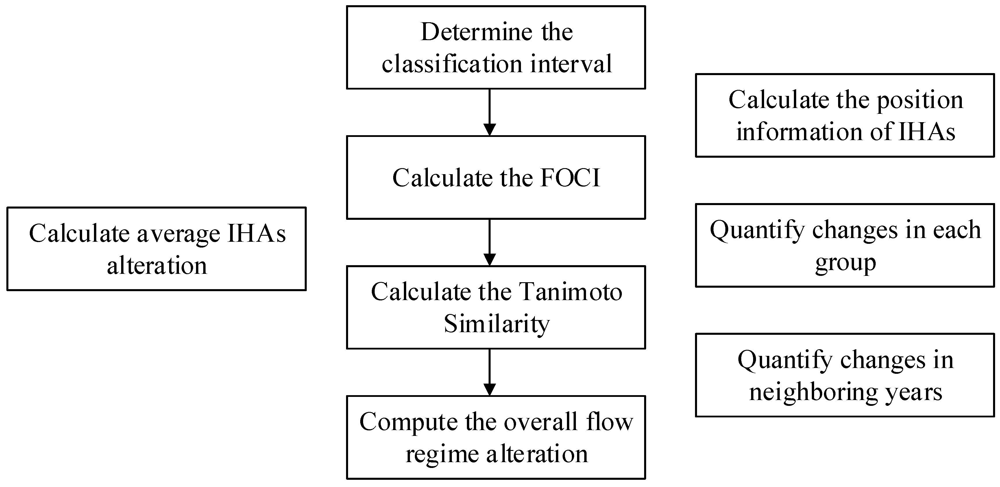
The overall procedure for the revised RVA method involves the following (Figure 1): (1) using the traditional RVA method to calculate each indicator alteration (IA; lateral alteration); (2) using the Tanimoto similarity method to calculate the Tanimoto similarity (TS; longitudinal alteration) coefficient, which is calculated via a first-order connectivity index; (3) calculating the change in TS between the pre- and post-impact period; and (4) calculating the overall flow regime alteration (OA; comprising both lateral and longitudinal alterations).
2.1. First-Order Connectivity Index
In order to compare the changes in each ICOHY, the similarity between two data series (pre- and post-impact series) must be analyzed. If the differences between the pre- and post-impact series are large, the similarity between the series is low. Various methods are available for calculating similarity, such as the Euclidean distance, general linear programing norm, and time warping [36,37,38]; these methods can be used to calculate the similarity between two times sequences with high precision. However, in order to first calculate the position information of each parameter, the FOCI method combined with the Tanimoto similarity should be used to calculate flow regime alteration caused by ICOHY.
The FOCI method can translate the positional information of each index in comparison sets (pre- and post-impact series) to a numerical value according to the category of the index. Thus, the changes in indices in different categories can be calculated. The FOCI method has been widely used in image pixel comparison, gene sequence alignment, and for handling data series connection problems, but has seldom been used in flow data series calculations. Divide the flow data series in different ranges (L1 = [(p0, p25), L2 = (p25, p75), and L3 = (p75, p100)). Treat each range as a data series, and calculate the value of FOCI that reflects the position information of 32 IHA in each range. The first step in the FOCI calculation is the classification of set A (a1, a2, …, a32). Subsequently, the FOCI is calculated in the same category via
in which Idt (li) is the FOCI in category li, li is the classification interval, t is the year, and σi represents the position sequence of category li.
Taking, as an example, that hydrological indicators are 1, 8, 10, and 20 in the same category (l1) in 1969, the FOCI (Id1969 (l1)) in 1969 is
2.2. Tanimoto Similarity
The Tanimoto similarity method is frequently used to compare the similarity of two gene sequences [39]; it is based on the Jacobian determinant and has wide range of applications in genetic engineering [40]. The Tanimoto similarity can be used to compare two data series in order to measure the similarity of FOCI in given years; the Tanimoto similarity coefficient () between years T1 and T2 is
in which is the similarity between T1 and T2, and IdT1 (li) is the FOIC in category li during T1.
When the value of TS is close to 1, the discrepancies between the two sets of hydrological indicators are negligible. Greater similarity indicates less hydrological alteration, which means less impact on the ecological environment. Lower TS values indicate greater ecological environment impact and suggest that action may be necessary to counteract the alteration.
2.3. Revised RVA Method
The difference between two data series can be calculated using the FOCI combined with the TS method, and this difference can reflect inherent characteristics of the hydrological alteration. The detailed procedure is as follows:
Step 1: Determine the classification interval
The traditional RVA method treats the 25th and 75th percentile values of the pre-impact period as the management target range; our revised RVA method uses the same range to determine the management target. The pre-impact series is P, and the post-impact series is Q, in which Pk1 = {p1k1, p2k1, …, pjk1, …, pmk1} and Qk2 = {p1k2, p2k2, …, pjk2, …, pmk2} (j = 1, 2, …, m; k1 = 1, 2, …, a, k2 = 1, 2, …, b). There are n assessment years and m hydrological evaluation indicators (m = 32). Then, the classification interval li (i = 3) can be divided into three ranges, L1 = (p0, p25), L2 = (p25, p75), and L3 = (p75, p100). For example, if the mean flow value of a river in January has an IHA value of 1, and the 25th and 75th percentile values are 386 and 458 m3 s−1, then the comparative intervals are (0, 386), (386.75, 458), and (458, +).
Step 2: Calculate the FOCI
After determining the classification range of the data set, the FOCI of the ith classification interval in kth year is calculated as follows:
in which S is the total number of hydrological indicators falling into the classification interval i. It is important to note that S must be sorted before the calculation of the index.
Step 3: Calculate the Tanimoto similarity
Because the pre-impact and post-impact years may be different, it is necessary to transform the Tanimoto similarity calculation formula. The Tanimoto similarity must be calculated between the pre- and post-impact periods in order to compute the difference between the two-data series. The Tanimoto similarity can be expressed as follows; TA is the change in the Tanimoto similarity value.
Step 4: Compute the overall flow regime alteration
The overall flow regime alteration calculation should consider both the vertical and horizontal alterations in hydrological indicators. The revised RVA method combines the IA and TA values to compute the OA (Figure 2). The revised RVA incorporates the three following principles. (1) IA and TA both influence the ecological environment; IA affects one ecological species (e.g., variations in the number of high pulses per year (IA 25) can affect the oviposition of migratory fish), while TA can affect all of the species in this system; (2) IA and TA are equally important; (3) The overall degree of hydrologic change is influenced by IA and TA. Thus, the OA is expressed as
2.4. Ecological Limits of Hydrologic Alteration (ELOHA)
The ELOHA framework, which is used to find relationships between flow regime alteration and ecological responses in order to define environmental flow [41], includes four scientific steps: (1) building a hydrologic foundation, (2) classifying river types, (3) assessing flow alterations, and (4) determining flow-ecology relationships. Flow alteration assessment is central to the ELOHA framework. The accuracy of alteration assessment of flow regime in the ELOHA framework can be much improved by the revised RVA method, enhancing it to build more accurate linkage between ecological response and flow regime alteration.
3. Case Study
The Jinsha River, which is located in the upper reaches of the Yangtze River (Figure 3), has a total length of 2326 km; Jinsha River is generally divided into three sections: the upper (Yellow), the middle (Green), and the lower (Purple) Jinsha River. The Jinsha River mainstream begins in the eastern Geladan Snowy Mountain in the Tanggula Mountain range, from which snowmelt provides the main source of flow in the upper reaches. The population density is not large in the upper reaches of the Jinsha River, and there are no large hydraulic structures. Therefore, climate is the main factor inducing flow regime alteration in this region [42]. The upper reaches of the Jinsha River area have become warmer, with a mean temperature increase from 0.5 to 2 °C from 1993 to 2014 that has significantly altered the natural flow regime (Figure 4). The Shigu hydrological station is located in the junction of the upper and middle reaches of the Jinsha River. It has long flow data in Shigu hydrological station, which can facilitate us to verify the proposed method. In this study, the pre-impact series consists of daily flow data from 1971 to 1992, and the post-impact series consists of daily flow data from 1993 to 2014. Daily streamflow data during 1971–2014 for the Jinsha River mainstream were collected from the Shigu hydrological station.
4. Results and Discussion
4.1. Comparing the Results of the Traditional and Revised RVA Methods
To statistically characterize the flow regime from 1971 to 2014, the IHA values were calculated in each year. Under the revised method, IA and TA were calculated separately. The IA value for each year was calculated based on the traditional RVA method using IHA 7.0 (The Nature Conservancy, Arlington, VA, USA); TA was determined by the Tanimoto similarity method. The results obtained with the traditional RVA and the revised method, including the lateral classification between the pre- and post-impact periods, are summarized in Table 2. The OA was 50%, which is higher than the average IA (33%). This higher alteration value suggests that traditional RVA methods underestimate flow regime alteration; this underestimation is likely caused primarily by neglecting the connectivity between data sets for each specific year and the positional information pertaining to the changes in the 32 IHA.
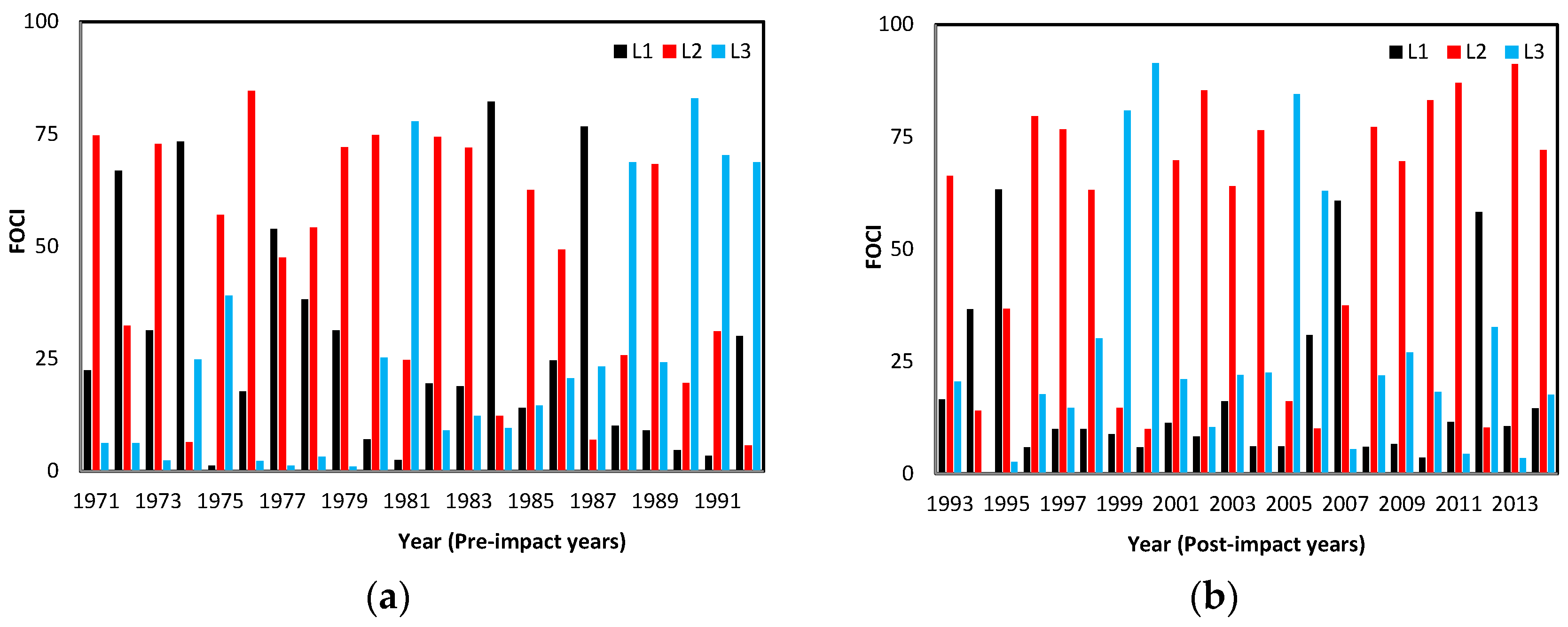
Based on Table 2, the number of IHA in three comparative intervals L1, L2, and L3 (L1 = (p0, p25), L2 = (p25, p75) and L3 = (p75, p100)) varies between years. For all years, the number of IHA is clearly higher in interval L2 than in the other two intervals. Furthermore, comparing the FOCI value in pre- and post-impact years (Figure 5), the FOCI values in interval L2 are almost always higher than those in the other two intervals. The change in FOCI values and numbers of IHA in each interval is consistent for most years, which indicates that the FOCI value effectively captures the characteristics of the 32 IHA within a given year. The change in IHA within each year is essential for determining particular flow regime characteristics and linking those characteristics to the aquatic ecosystem [43,44]. If only a few years are considered, the FOCI values and numbers of IHA become inconsistent, as the IHA reflect flow regime alterations jointly and the eco-response to each IHA is different [45,46]. Moreover, the position of each IHA must be considered in determining the FOCI value; therefore, in some years, the FOCI may be inconsistent with the number of IHA. The results show that the inclusion of IHA position and the number of IHA in each interval aids in the accurate estimation of flow regime alteration.
4.2. Sensitivity of IA and TA
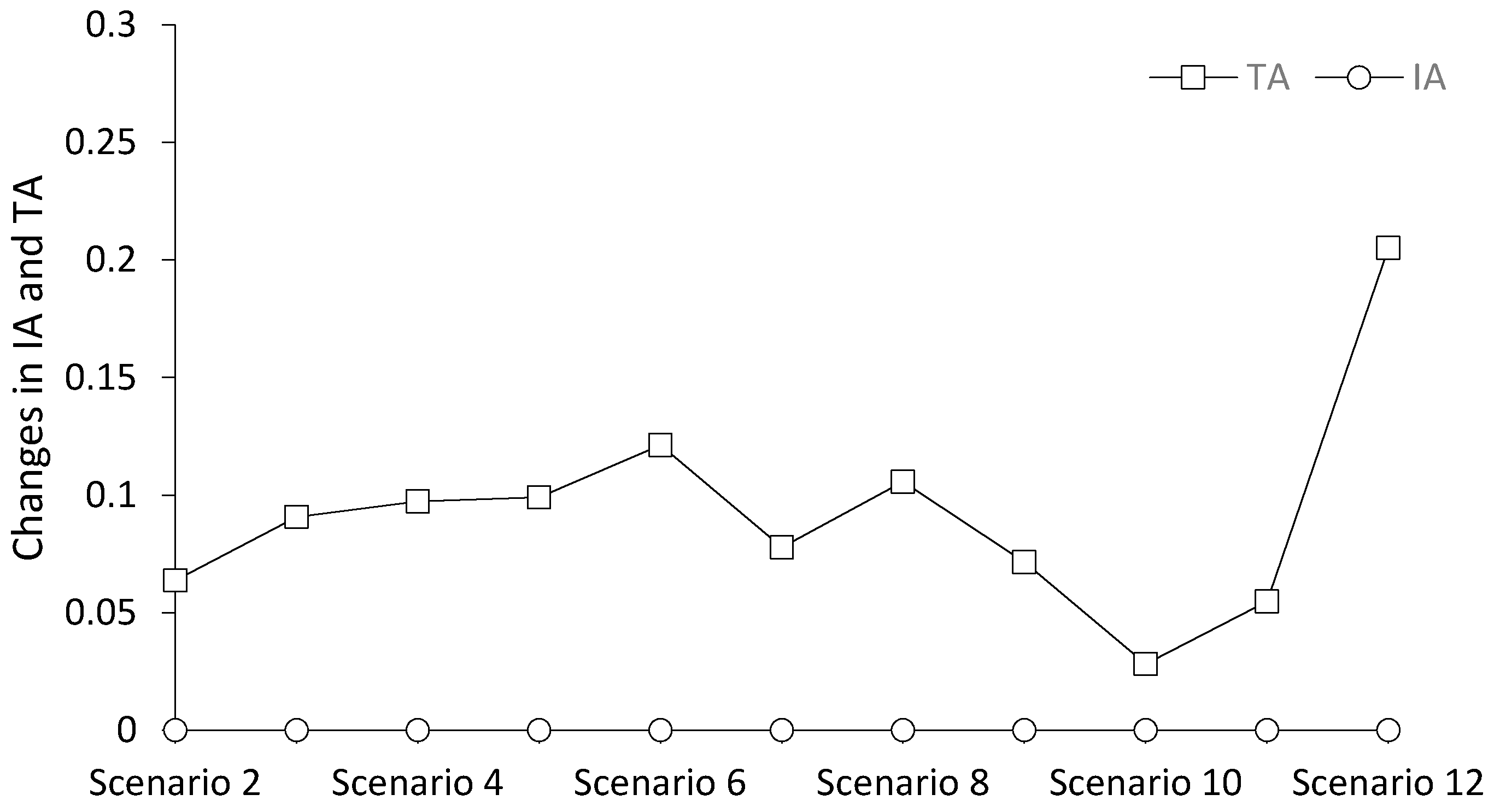
To determine the sensitivity of the revised RVA method, we designed 12 scenarios. The year of exchange was increased over an equidistant range of 2; the first term was 0 years, and the last term was 22 years. In scenario 1, we exchanged 0 years of IHA (exchange years = 0). In scenario 2, we exchanged the 1st and 22nd year IHA values (exchange years = 2). In scenario 3, we exchanged the 2nd and 21st year IHA values (exchange years = 4), and so on. In this manner, the changes in IA and OA were calculated for 12 scenarios. We used scenario 1 as a baseline from which to calculate the changes in IA and TA. The results are shown in Figure 6. The change in IA remains constant at 0 with increasing number of exchanges. However, the change in TA is never equal to 0. Indeed, changes in the time series order affect the flow regime and thus the response of local aquatic organisms, which in turn affect the maintenance of ecological functions; changes in the type of hydrological year (e.g., wet year to dry year) may cause reduced fish species abundance [47]. Changes in the IHA time series order can also cause extreme flows (i.e., droughts and floods) [48,49]. Thus, the flow regime alteration calculations must include changes in the IHA time series order. TA can reflect changes in the IHA time series order, and the revised RVA method takes the TA value into account; thus, the revised method reflects the actual hydrological alteration more accurately.
TA does not increase with increases in the number of exchanged years, which reflects the fact that changing the natural hydrological flow regime does not necessarily disrupt the ecological balance, because natural flow regimes can also cause extreme flow events. For instance, normal years can contain extreme low flow events, which can cause poorly developed bank top vegetation and reduced mesohabitat diversity [50]. Therefore, controlling natural flow regime, as well as peak shaving and valley filling, can help to maintain the health of the ecosystem. In scenario 10 (exchange years = 18), the change in TA is minimized, which indicates that the IHA time series order in scenario 10 is the closest to the baseline time series. In practice, we can determine the time series with the least TA change based on yearly flow data and incorporate this time series into the ELOHA framework.
4.3. Application of the Revised Method to the ELOHA Framework
Flow regime alteration is often assessed in order to generate preliminary flow-ecology relationships for use in riverine restoration with ELOHA. The changes in IHA in each group represent the influence of each aspect of flow regime (i.e., magnitude, frequency, duration, time, and rate, as shown in Table 1) in the ecosystem. Lower degrees of IHA alteration in given groups represent weaker ecosystem influences [51]. Therefore, we used the revised RVA method to assess the influence of flow regime alteration on ecosystem response.
IA, TA, and OA results calculated using the revised RVA method are shown in Figure 7. In the OA analysis, group 5 (rate and frequency of water condition changes) is found to undergo the greatest alteration. The changes to group 5 can affect the ability of plant roots to maintain contact with the phreatic water supply. If the regional plants are not adaptable to drought conditions, management measures must be developed to prevent drought. This results in more stable population sizes that rarely go extinct by increasing flood frequency properly [52]. The TA value indicates the changes in the ICOHY and the IHA positions. In the TA analysis, groups 1 and 2 feature the largest values. The changes in group 1 will affect the availability of aquatic habitat, and the alterations in group 2 will affect the distribution of plant communities. These results suggest that the alteration of hydrological year types in this area will significantly affect aquatic habitats and plant community distributions. Furthermore, some indicators in groups 1 and 2 have strong correlations with aquatic habitat or plant community distribution [53,54,55].
Based on the analysis of the preliminary flow-ecology relationships in each group (Table 1), the following recommendations can be made for the implementation of the ELOHA framework in the Jinsha River: (1) Generate plant species statistics in the region and identify plant species with high water dependence; then, develop appropriate conservation strategies to ensure the healthy development of such plants. (2) Examine the habitat of aquatic organisms; find the number and species of aquatic organisms in the region that are dependent on the aquatic habitat and develop habitat conservation strategies to ensure healthy aquatic habitat for regional organisms. (3) Generate plant community distribution statistics for the region. Determine the relationship between the plant community distribution and flow regime alteration and develop efficient measures to retain the plant community distribution.
4.4. Model Limitations
The accuracy of the traditional RVA method can be significantly improved by accounting for the FOCI and Tanimoto similarity. However, the revised RVA method is still limited by the lack of measured ecological data [56]. The revised RVA method considers the impacts of the 32 IHA factors to be equal; however, in reality, the ecological impacts of the indicators are usually different. Therefore, accurate ecological data are required to properly calculate the proportional contribution of each index to the FOCI. The index that is used for the protection target should have a greater influence on the proportion of the increase than the target index. If these conditions are satisfied, the calculated results can reflect the actual situation and provide more accuracy and services to the ELOHA framework [57,58].
The revised RVA method is a significant improvement over the traditional RVA method. This method can effectively calculate flow regime alteration simply and quickly in areas lacking measured data, thereby saving computation costs; it can also be used by management authorities to produce feasible management plans. Nevertheless, the revised RVA method does not contain a feedback model; thus, after measurements are assumed, there is no feedback mechanism to substantiate the true flow-ecological response relationship. Feedback information can be used to increase the accuracy of the revised RVA estimates and also affects the promotion of the revised RVA method to a certain extent. Thus, future research will focus on the inclusion of a feedback model in the revised RVA method.
5. Conclusions
This work presents a revised RVA method for flow regime alteration determination that incorporates the ICOHY and positional information for the 32 IHA relevant to natural flow regimes. Two major conclusions are drawn herein. First, the values of TA and IA reflect the preliminary flow-ecology relationships that are important to riverine restoration and can be used to enhance the ELOHA framework. Second, a case study concerning the upper reaches of the Yangtze River suggests that the traditional RVA method underestimates flow alteration, because it neglects the ICOHY and the IHA positional information; the revised method adequately characterizes the hydrologic regime and enables a more comprehensive analysis of flow regime alteration.
Author Contributions
Wenqi Peng provided overall guidance; Wei Huang and Xiaodong Qu analyzed the data; Shailesh Kumar Singh contributed analysis tools; Jinjin Ge wrote the paper.
Funding
This research was funded by the National Key Project R and D Program of China (Grant Nos. 2017YFC0404506 and 2016YFC0401709), the major Science and Technology Program for Water Pollution Control and Treatment (2017ZX07301003), National Natural Science Foundation of China (Grant Nos. 51309253, 51439007, and 51479219), and the IWHR Research and Development Support Program (Grant Nos. WE0145B532017, WE0145B782017, WE0145B342016, and WE0145B592017).
Conflicts of Interest
The authors declare no conflict of interest.
References
- Bunn, S.E.; Arthington, A.H. Basic principles and ecological consequences of altered flow regimes for aquatic biodiversity. Environ. Manag. 2002, 30, 492–507. [Google Scholar] [CrossRef]
- Li, D.N.; Long, D.; Zhao, J.; Lu, H.; Hong, Y. Observed changes in flow regimes in the Mekong River Basin. J. Hydrol. 2017, 551, 217–232. [Google Scholar] [CrossRef]
- Poff, L.R.; Matthews, J.H. Environmental flows in the anthropocence: Past progress and future prospects. Curr. Opin. Environ. Sustain. 2013, 5, 667–675. [Google Scholar] [CrossRef]
- Arthington, A.H. Environmental flows: A scientific resource and policy framework for river conservation and restoration. Aquat. Conserv. 2015, 25, 155–161. [Google Scholar] [CrossRef]
- Arthington, A.H.; Naiman, R.J.; Mcclain, M.E.; Nilsson, C. Preserving the biodiversity and ecological services of rivers: New challenges and research opportunities. Freshw. Biol. 2010, 55, 1–16. [Google Scholar] [CrossRef]
- Arthington, A.H. Environmental flows: Ecological limits of hydrologic alteration (ELOHA). In The Wetland Book; Finlayson, C.M., Everard, M., Irvine, K., McInnes, R.J., Middleton, B.A., van Dam, A.A., Davidson, N.C., Eds.; Springer: Dordrecht, The Netherlands, 2016; pp. 1–5. [Google Scholar]
- Buchanan, C.; Moltz, H.L.N.; Haywood, H.C.; Palmer, J.B.; Griggs, A.N. A test of the ecological limits of hydrologic alteration (ELOHA) method for determining environmental flows in the Potomac River basin, U.S.A. Freshw. Biol. 2013, 58, 2632–2647. [Google Scholar] [CrossRef]
- Solans, M.A.; de Jalón, G.D. Basic tools for setting environmental flows at the regional scale: Application of the ELOHA framework in a Mediterranean river basin. Ecohydrology 2016, 9, 1517–1538. [Google Scholar] [CrossRef]
- Yang, Z.; Yan, Y.; Liu, Q. Assessment of the flow regime alterations in the lower Yellow River, China. Ecol. Inform. 2012, 10, 56–64. [Google Scholar] [CrossRef]
- Botter, G.; Basso, S.; Porporato, A.; Rodriguez-Iturbe, I.; Rinaldo, A. Natural streamflow regime alterations: Damming of the Piave river basin (Italy). Water Resour. Res. 2010, 46, 1896–1911. [Google Scholar] [CrossRef]
- Tang, J.; Yin, X.A.; Yang, P.; Yang, Z.F. Climate-induced flow regime alterations and their implications for the Lancang River, China. River Res. Appl. 2015, 31, 422–432. [Google Scholar] [CrossRef]
- Yang, T.; Cui, T.; Xu, C.Y.; Ciais, P.; Shi, P. Development of a new IHA method for impact assessment of climate change on flow regime. Glob. Planet. Chang. 2017, 156, 68–79. [Google Scholar] [CrossRef]
- Mittal, N.; Bhave, A.G.; Mishra, A.; Singh, R. Impact of human intervention and climate change on natural flow regime. Water Res. Manag. 2016, 30, 685–699. [Google Scholar] [CrossRef] [Green Version]
- Yang, Y.; Yang, Z.; Yin, X.A.; Liu, Q. A framework for assessing flow regime alterations resulting from the effects of climate change and human disturbance. Hydrol. Sci. J. 2018, 63, 1–16. [Google Scholar] [CrossRef]
- Xue, L.; Zhang, H.; Yang, C.; Zhang, L.; Sun, C. Quantitative assessment of hydrological alteration caused by irrigation projects in the Tarim River basin, China. Sci. Rep. 2017, 7, 4291. [Google Scholar] [CrossRef] [PubMed]
- Kim, B.S.; Kim, B.K.; Kwon, H.H. Assessment of the impact of climate change on the flow regime of the Han river basin using indicators of hydrologic alteration. Hydrol. Processes 2015, 25, 691–704. [Google Scholar] [CrossRef]
- Olden, J.D.; Poff, N.L. Redundancy and the choice of hydrologic indices for characterizing streamflow regimes. River Res. Appl. 2010, 19, 101–121. [Google Scholar] [CrossRef]
- Stanford, J.A.; Ward, J.V.; Liss, W.J.; Frissell, C.A.; Williams, R.N.; Lichatowich, J.A.; Richter, B.D.; Baumgartner, J.V.; Powell, J.; Braun, D.P. A method for assessing hydrologic alteration within ecosystems. Conserv. Biol. 1996, 10, 1163–1174. [Google Scholar]
- Richter, B.; Baumgartner, J.; Wigington, R.; Braun, D. How much water does a river need? Freshw. Biol. 1997, 37, 231–249. [Google Scholar] [CrossRef]
- Zhang, Q.; Xiao, M.; Liu, C.L.; Singh, V.P. Reservoir-induced hydrological alterations and environmental flow variation in the East River, the Pearl River basin, China. Stoch. Environ. Res. Risk Assess. 2014, 28, 2119–2131. [Google Scholar] [CrossRef]
- Galat, D.L.; Lipkin, R. Restoring ecological integrity of great rivers: Historical hydrographs aid in defining reference conditions for the Missouri River. In Assessing the Ecological Integrity of Running Waters; Springer: Dordrecht, The Netherlands, 2000; pp. 29–48. [Google Scholar]
- Shen, C.; Dong, L.H.; Wang, Y.C.; Feng, S.X.; Wang, Y. Trend analysis on the flow alteration in the nature reserve, upstream of Yangtze river. Appl. Mech. Mater. 2014, 641, 132–136. [Google Scholar] [CrossRef]
- Mathews, R.; Richter, B.D. Application of the indicators of hydrologic alteration software in environmental flow setting. J. Am. Water Res. Assoc. 2007, 43, 1400–1413. [Google Scholar] [CrossRef]
- Shiau, J.T.; Wu, F.C. A histogram matching approach for assessment of flow regime alteration: Application to environmental flow optimization. River Res. Appl. 2008, 24, 914–928. [Google Scholar] [CrossRef]
- Belmar, O.; Bruno, D.; Martínez-Capel, F.; Barquín, J.; Josefa Velasco, J. Effects of flow regime alteration on fluvial habitats and riparian quality in a semiarid Mediterranean basin. Ecol. Indic. 2013, 30, 52–64. [Google Scholar] [CrossRef]
- Richter, B.D.; Baumgartner, J.V.; Braun, D.P.; Powell, J. A spatial assessment of hydrologic alteration within a river network. River Res. Appl. 1998, 14, 329–340. [Google Scholar] [CrossRef]
- Richter, B.D.; Warner, A.T.; Meyer, J.L.; Lutz, K. A collaborative and adaptive process for developing environmental flow recommendations. River Res. Appl. 2006, 22, 297–318. [Google Scholar] [CrossRef]
- Lytle, D.A.; Merritt, D.M. Hydrologic regimes and riparian forests: A structured population model for cottonwood. Ecology 2004, 85, 2493–2503. [Google Scholar] [CrossRef]
- Shiau, J.T.; Wu, F.C. Pareto-optimal solutions for environmental flow schemes incorporating the intra-annual and interannual variability of the natural flow regime. Water Resour. Res. 2007, 43. [Google Scholar] [CrossRef]
- Yin, X.A.; Yang, Z.F.; Petts, G.E. A new method to assess the flow regime alterations in riverine ecosystems. River Res. Appl. 2015, 31, 497–504. [Google Scholar] [CrossRef]
- Yu, C.; Yin, X.; Yang, Z. A revised range of variability approach for the comprehensive assessment of the alteration of flow regime. Ecol. Eng. 2016, 96, 200–207. [Google Scholar] [CrossRef]
- Caporossi, G.; Gutman, I.; Hansen, P.; Pavlović, L. Graphs with maximum connectivity index. Comput. Biol. Chem. 2003, 27, 85–90. [Google Scholar] [CrossRef]
- Randić, M. The connectivity index 25 years after. J. Mol. Graph. Model. 2001, 20, 19–35. [Google Scholar] [CrossRef]
- Kryszkiewicz, M. Bounds on lengths of real valued vectors similar with regard to the Tanimoto similarity. In Proceedings of the Asian Conference on Intelligent Information and Database Systems, Kuala Lumpur, Malaysia, 18–20 March 2013; pp. 445–454. [Google Scholar]
- Zhang, B.; Vogt, M.; Maggiora, G.M.; Bajorath, J. Design of chemical space networks using a Tanimoto similarity variant based upon maximum common substructures. J. Comput-Aided Mol. Des. 2015, 29, 937–950. [Google Scholar] [CrossRef] [PubMed]
- Goldin, D.Q.; Millstein, T.D.; Kutlu, A. Bounded similarity querying for time-series data. Inf. Comput. 2004, 194, 203–241. [Google Scholar] [CrossRef]
- Keogh, E. Efficiently finding arbitrarily scaled patterns in massive time series databases. In Proceedings of the European Conference on Principles of Data Mining and Knowledge Discovery, Cavtat-Dubrovnik, Croatia, 22–26 September 2003; pp. 253–265. [Google Scholar]
- Lee, S.; Kwon, D.; Lee, S. Minimum distance queries for time series data. J. Syst. Softw. 2004, 69, 105–113. [Google Scholar] [CrossRef]
- Tuna, S.; Niranjan, M. Classification with binary gene expressions. J. Biomed. Sci. Eng. 2009, 2, 390–399. [Google Scholar] [CrossRef]
- Fligner, M.A.; Verducci, J.S.; Blower, P.E. A modification of the Jaccard–Tanimoto similarity index for diverse selection of chemical compounds using binary strings. Technometrics 2002, 44, 110–119. [Google Scholar] [CrossRef]
- McManamay, R.A.; Orth, D.J.; Dolloff, C.A.; Mathews, D.C. Application of the ELOHA framework to regulated rivers in the Upper Tennessee River Basin: A case study. Environ. Manag. 2013, 51, 1210–1235. [Google Scholar] [CrossRef] [PubMed]
- Liu, H.; Lan, H.; Liu, Y.; Zhou, Y. Characteristics of spatial distribution of debris flow and the effect of their sediment yield in main downstream of Jinsha River, China. Environ. Earth Sci. 2009, 64, 1653–1666. [Google Scholar] [CrossRef]
- Lee, A.; Cho, S.; Kang, D.K.; Kim, S. Analysis of the effect of climate change on the Nakdong River stream flow using indicators of hydrological alteration. J. Hydro-Environ. Res. 2014, 8, 234–247. [Google Scholar] [CrossRef]
- Rolls, R.J.; Arthington, A. How do low magnitudes of hydrologic alteration impact riverine fish populations and assemblage characteristics? Ecol. Indic. 2014, 39, 179–188. [Google Scholar] [CrossRef]
- Rahman, M.A.T.M.T.; Hoque, S.; Saadat, A.H.M. Selection of minimum indicators of hydrologic alteration of the Gorai River, Bangladesh using principal component analysis. Sustain. Water Res. Manag. 2017, 3, 13–23. [Google Scholar] [CrossRef]
- Yu, C.; Yin, X.; Yang, Z.; Dang, Z. Assessment of the degree of hydrological indicators alteration under climate change. In Proceedings of the 6th International Conference on Energy and Environmental Protection, Zhuhai, China, 29–30 June 2017; pp. 13–20. [Google Scholar]
- Jowett, I.G.; Richardson, J.; Bonnett, M.L. Relationship between flow regime and fish abundances in a gravel-bed river, New Zealand. J. Fish Biol. 2005, 66, 1419–1436. [Google Scholar] [CrossRef]
- Marcinkowski, P.; Grygoruk, M. Long-term downstream effects of a dam on a lowland river flow regime: Case study of the Upper Narew. Water 2017, 9, 783. [Google Scholar] [CrossRef]
- Seyam, M.; Othman, F. Long-term variation analysis of a tropical river’s annual streamflow regime over a 50-year period. Theor. Appl. Climatol. 2015, 121, 71–85. [Google Scholar] [CrossRef]
- Belmar, O.; Velasco, J.; Gutiérrez-Cánovas, C.; Millán, A.; Wood, P.J. The influence of natural flow regimes on macroinvertebrate assemblages in a semiarid Mediterranean basin. Ecohydrology 2012, 6, 363–379. [Google Scholar] [CrossRef] [Green Version]
- You, J.Y.; Thum, B.H.; Lin, F.H. The examination of reproducibility in hydro-ecological characteristics by daily synthetic flow models. J. Hydrol. 2014, 511, 904–919. [Google Scholar] [CrossRef]
- Johnson, W.C. Riparian vegetation diversity along regulated rivers: Contribution of novel and relict habitat. Freshw. Biol. 2002, 47, 749–759. [Google Scholar] [CrossRef]
- Nilsson, C.; Berggren, K. Alterations of riparian ecosystems caused by river regulation: Dam operations have caused global-scale ecological changes in riparian ecosystems. How to protect river environments and human needs of rivers remains one of the most important questions of our time. BioScience 2000, 50, 783–792. [Google Scholar]
- Doyle, M.W.; Stanley, E.H.; Strayer, D.L.; Jacobson, R.B.; Schmidt, J.C. Effective discharge analysis of ecological processes in streams. Water Resour Res. 2005, 41. [Google Scholar] [CrossRef]
- Timpe, K.; Kaplan, D. The changing hydrology of a dammed Amazon. Sci. Adv. 2017, 3, e1700611. [Google Scholar] [CrossRef] [PubMed]
- Ardron, J.A. Three initial OSPAR tests of ecological coherence: Heuristics in a data-limited situation. Ices J. Mar. Sci. 2008, 65, 1527–1533. [Google Scholar] [CrossRef]
- Macnaughton, C.J.; Mclaughlin, F.; Bourque, G.; Senay, C.; Lanthier, G. The effects of regional hydrologic alteration on fish community structure in regulated rivers. River Res. Appl. 2017, 33, 249–257. [Google Scholar] [CrossRef]
- Williams, J.G. Building hydrologic foundations for applications of ELOHA: How long a record should you have? River Res. Appl. 2018, 34, 93–98. [Google Scholar] [CrossRef]
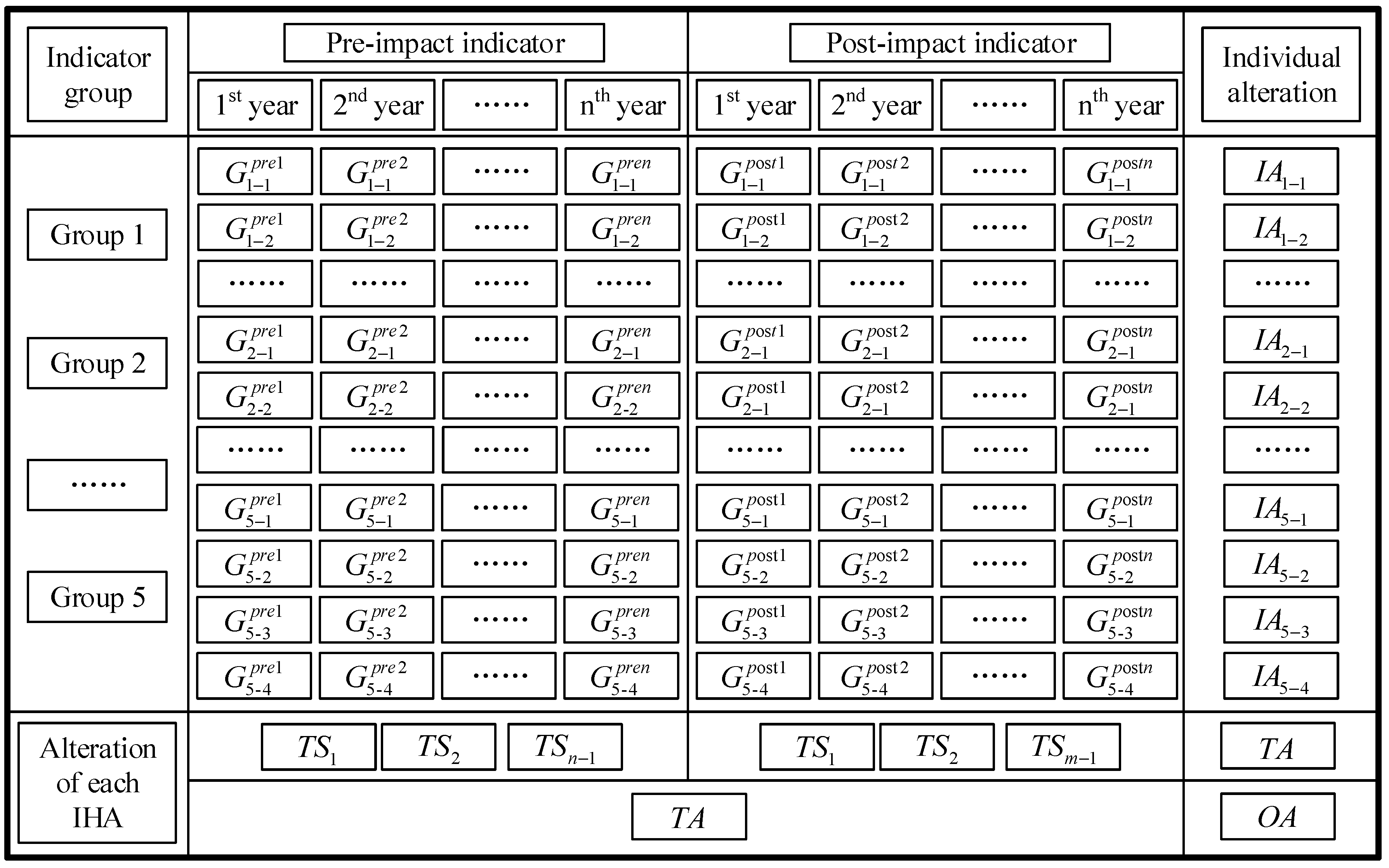
Figure 1.
Main idea of the revised range of variability approach (RVA) method.

Figure 2.
Flow chart of the methodology adopted in this study. The left side shows the single step in the traditional RVA, while the right-hand boxes show the novel steps in the current study.
Figure 2.
Flow chart of the methodology adopted in this study. The left side shows the single step in the traditional RVA, while the right-hand boxes show the novel steps in the current study.

Figure 3.
Location of the study area.

Figure 4.
Mean annual flow at Shigu station from 1971 to 2014 (since 1992, the average flow has shifted from 1298 to 1362 m3 s−1).
Figure 4.
Mean annual flow at Shigu station from 1971 to 2014 (since 1992, the average flow has shifted from 1298 to 1362 m3 s−1).

Figure 5.
ICOHY of three comparative intervals in pre- and post-impact years (the pre-impact series consists of daily flow data from 1971 to 1992 and the post-impact series consists of daily flow data from 1993 to 2014). (a) Alteration in pre-impact period and (b) Alteration in post-impact period.
Figure 5.
ICOHY of three comparative intervals in pre- and post-impact years (the pre-impact series consists of daily flow data from 1971 to 1992 and the post-impact series consists of daily flow data from 1993 to 2014). (a) Alteration in pre-impact period and (b) Alteration in post-impact period.

Figure 6.
Changes in IA and TA under different numbers of exchanged years.

Figure 7.
Changes in IHA groups under IA, TA, and OA.


| IHA Statistical Group | Ecosystem Influences | Hydrologic Parameters |
|---|---|---|
| Group 1: Magnitude of monthly water conditions | Availability of aquatic habitat | Mean flow for each calendar month |
| Group 2: Magnitude and duration of annual extreme flow | Distribution of plant communities in lakes, ponds, and floodplains | Annual minimum 1-day, 3-day, 7-day, 30-day, and 90-day means |
| Annual maximum 1-day, 3-day, 7-day, 30-day, and 90-day means | ||
| Group 3: Timing of annual extreme water conditions | Spawning cues for migratory fish | Date of annual 1-day maximum flow |
| Date of annual 1-day minimum flow | ||
| Group 4: Frequency and duration of high and low pulses | Water bird feeding, resting, and breeding | Number of high pulses in each year |
| Number of low pulses in each year | ||
| Mean duration of the annual high pulse | ||
| Mean duration of the annual low pulse | ||
| Group 5: Rate and frequency of water condition changes | Drought stress on plants | Rise rates: Mean or median of all positive differences between consecutive daily values |
| Fall rates: Mean or median of all negative differences between consecutive daily values | ||
| Number of rises | ||
| Number of falls |
Table 2.
Summary of the degree of hydrologic alteration and IHA classification information (bold text indicates that the FOCI value in interval L2 is higher than those in the other two intervals).
Table 2.
Summary of the degree of hydrologic alteration and IHA classification information (bold text indicates that the FOCI value in interval L2 is higher than those in the other two intervals).
| Pre-Impact Series | Post-Impact Series | ||||||
|---|---|---|---|---|---|---|---|
| Year | L1 | L2 | L3 | Year | L1 | L2 | L3 |
| 1971 | 10 | 17 | 5 | 1993 | 9 | 12 | 11 |
| 1972 | 16 | 12 | 5 | 1994 | 18 | 7 | 6 |
| 1973 | 14 | 15 | 3 | 1995 | 14 | 17 | 2 |
| 1974 | 18 | 4 | 11 | 1996 | 6 | 19 | 7 |
| 1975 | 3 | 18 | 10 | 1997 | 7 | 19 | 6 |
| 1976 | 8 | 22 | 2 | 1998 | 8 | 10 | 14 |
| 1977 | 15 | 16 | 2 | 1999 | 7 | 9 | 15 |
| 1978 | 10 | 18 | 4 | 2000 | 6 | 6 | 19 |
| 1979 | 13 | 18 | 1 | 2001 | 4 | 18 | 10 |
| 1980 | 7 | 12 | 13 | 2002 | 4 | 21 | 7 |
| 1981 | 3 | 13 | 15 | 2003 | 8 | 13 | 11 |
| 1982 | 8 | 17 | 7 | 2004 | 6 | 16 | 10 |
| 1983 | 10 | 16 | 6 | 2005 | 6 | 7 | 18 |
| 1984 | 19 | 10 | 4 | 2006 | 15 | 5 | 11 |
| 1985 | 8 | 18 | 7 | 2007 | 13 | 14 | 6 |
| 1986 | 11 | 16 | 5 | 2008 | 6 | 18 | 8 |
| 1987 | 16 | 7 | 10 | 2009 | 5 | 14 | 13 |
| 1988 | 7 | 12 | 12 | 2010 | 4 | 21 | 7 |
| 1989 | 7 | 16 | 9 | 2011 | 7 | 22 | 3 |
| 1990 | 5 | 11 | 15 | 2012 | 15 | 4 | 14 |
| 1991 | 5 | 10 | 16 | 2013 | 7 | 21 | 4 |
| 1992 | 14 | 6 | 11 | 2014 | 8 | 14 | 10 |
| IA | 33% | ||||||
| TA | 25% | ||||||
| OA | 50% | ||||||
© 2018 by the authors. Licensee MDPI, Basel, Switzerland. This article is an open access article distributed under the terms and conditions of the Creative Commons Attribution (CC BY) license (http://creativecommons.org/licenses/by/4.0/).
Share and Cite
MDPI and ACS Style
Ge, J.; Peng, W.; Huang, W.; Qu, X.; Singh, S.K. Quantitative Assessment of Flow Regime Alteration Using a Revised Range of Variability Methods. Water 2018, 10, 597. https://doi.org/10.3390/w10050597
AMA Style
Ge J, Peng W, Huang W, Qu X, Singh SK. Quantitative Assessment of Flow Regime Alteration Using a Revised Range of Variability Methods. Water. 2018; 10(5):597. https://doi.org/10.3390/w10050597
Chicago/Turabian StyleGe, Jinjin, Wenqi Peng, Wei Huang, Xiaodong Qu, and Shailesh Kumar Singh. 2018. "Quantitative Assessment of Flow Regime Alteration Using a Revised Range of Variability Methods" Water 10, no. 5: 597. https://doi.org/10.3390/w10050597
Note that from the first issue of 2016, this journal uses article numbers instead of page numbers. See further details here.