Assessing the Influence of Precipitation on Shallow Groundwater Table Response Using a Combination of Singular Value Decomposition and Cross-Wavelet Approaches

Abstract

Identifying the spatiotemporal change of the groundwater table to precipitation at the river basin scale can be important for regional water resource management. In this study, we proposed a method that combines singular value decomposition and cross-wavelet approaches to analyze the relationship between groundwater level dynamics and precipitation. The method was applied to the Naoli River Basin, Northeast China. Moreover, the method of continuous wavelet using fast Fourier transform was also used to reveal clearly the relationship between groundwater level and heavy precipitation. The results showed that the major mode of relationship between groundwater and precipitation was divided into four patterns in the study area. In general, the lag time is 27.4 (standard deviation: ±8.1) days in pattern 1, 107.5 (standard deviation: ±13.2) days in pattern 2, 139.9 (standard deviation: ±11.2) days in pattern 3, and 173.4 (standard deviation: ±20.3) days in pattern 4, respectively. In addition, the response of groundwater level dynamics is very sensitive to heavy precipitation in all patterns. Therefore, enhancing the utilization of heavy rainfall and flood resources is an effective way to increase groundwater recharge in this basin.

1. Introduction

Groundwater is a vital freshwater source for a variety of domestic, agricultural, and industrial uses [1,2]. In the past several decades, depletion of groundwater storage has emerged all over the world because of the excessive increase of groundwater use for rapid development in agriculture, industry, and urbanization [3], for instance, in India [4], the United States [5], Australia [6], Africa [7], and China [8,9]. The situation of groundwater shortage in many countries continues, threatening the long-term sustainability of the regional economy and ecosystem services.

Precipitation infiltration is one of the major sources for local groundwater recharge. Although there have been many studies on groundwater recharge, our knowledge about the direct response of local groundwater table to precipitation is still limited. Furthermore, it is necessary to study the spatiotemporal change of the precipitation–groundwater table relation in the context of climate change and high-intensity human activities [10,11,12]. Therefore, the patterns of spatiotemporal responses should be investigated, which will be helpful for groundwater management and its sustainable use [10,13]. The singular value decomposition (SVD) analysis is one of the commonly used methods for statistical analysis of the coupling of two variable fields, which can make singular value decomposition of the cross-coefficient matrix of the two variable fields. The results can be used to explain the covariance structure of the variable fields in space. The method has been widely used in meteorology to determine the relationship between precipitation and atmospheric circulation indexes [14,15,16,17,18]. Since the method can describe co-variability modes between two variable fields [19,20], it can be used for identifying the complex spatial response modes of groundwater level to precipitation. To determine the temporal relationships between groundwater and precipitation, the cross-wavelet transform (XWT) and wavelet coherence (WTC) can be used for examining the common power and their phase relationships in time–frequency spaces [21,22]. This method has been widely used in the fields of hydrology and meteorology [23,24,25]. In addition, the phase angles can also be applied to calculate the temporal lags in the response of groundwater level dynamics to precipitation. Therefore, this method combining SVD and cross-wavelet approaches can quickly identify the spatiotemporal relationship between groundwater level dynamics and precipitation.

This study aimed to develop a new approach combining the SVD method and cross-wavelet approach to identify the spatiotemporal patterns in the response of shallow groundwater table dynamics to precipitation. Furthermore, this method was applied to the case study area, the Naoli River Basin of Northeast China, and the factors influencing the spatiotemporal response pattern between two time series were demonstrated in detail.

2. Materials and Methods

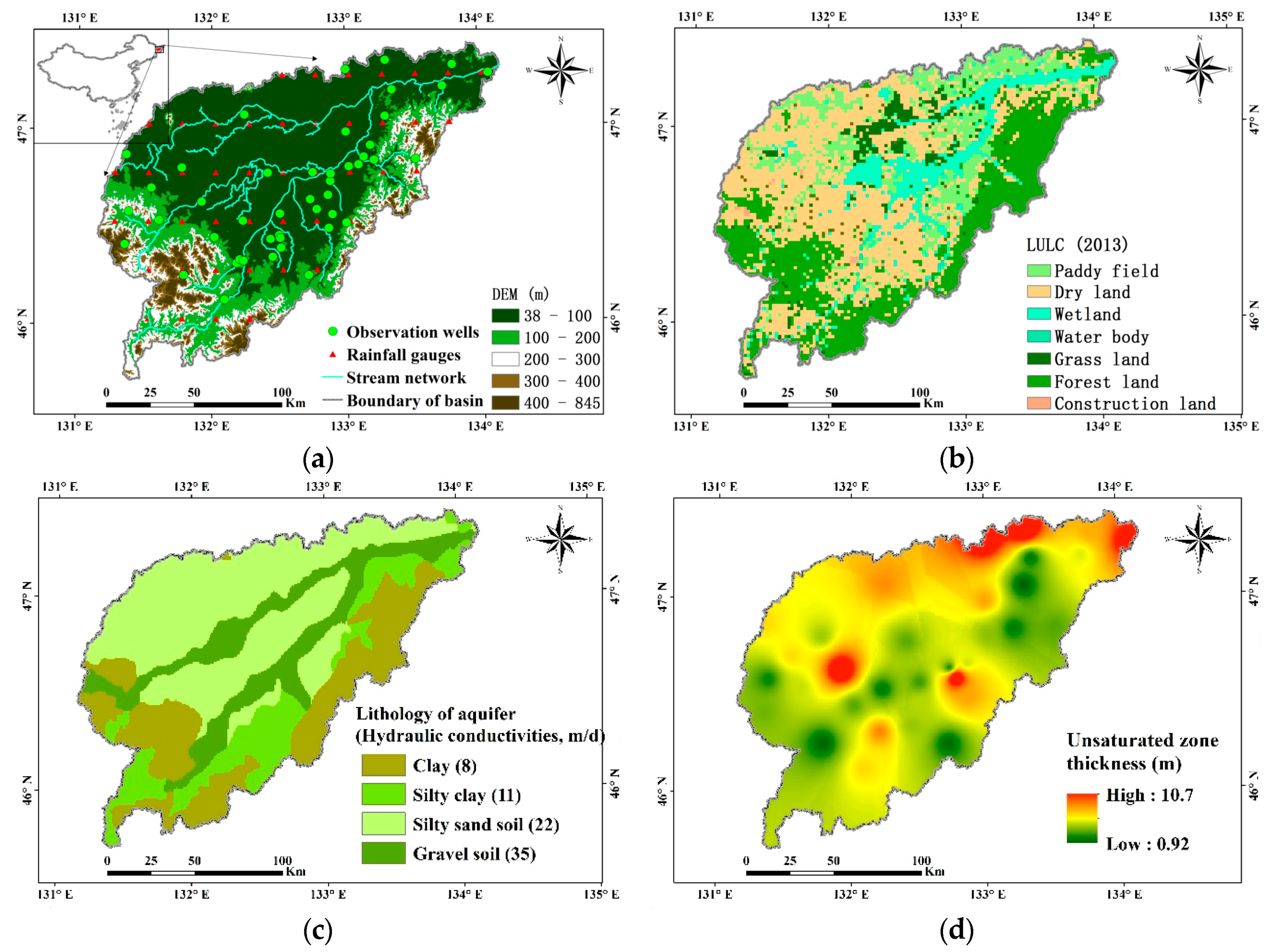
2.1. Study Area

The Naoli River Basin (45°43′–47°35′ N and 131°31′–134°10′ E) located in China’s high-latitude northeast covers a total land area of approximately 24,200 km². It is one of the most important grain production bases in China, as well as a large inland freshwater wetland region (Figure 1). Climate of this basin can be characterized as temperate humid and semihumid continental monsoon, with a long-term annual average temperature of 3.5 °C and a long-term annual average precipitation of 518 mm, 60–72% of which falls during May and September. The terrain of this area is flat, and most of the area is located in the floodplain with a gradient of 0% to 3%. Land use and land cover (LULC) of the Naoli River Basin have changed considerably in the past decade. The basin used to have a large area of wetlands, but a majority of them (i.e., about 80%) were converted into cultivated land during the past half century [26]. Currently, major LULC types in the basin include paddy field, dry land, forest land, grass land, wetland, construction land, and water body (Figure 1b). The paddy fields occupy 22.7% (or 5500 km²), dry lands 35.1% (or 8500 km²), the forest lands 25.3% (or 6100 km²), the grass lands 2.6% (or 600 km²) [26], wetlands 9.8% (or 2400 km²), and others 4.5% (or 1100 km²). The basin is mainly covered by Quaternary alluvial sediments, where the largest amount of groundwater storage and extraction are located. The lithology and hydraulic conductivities of the aquifers are clay (8 m/day), silty clay (11 m/day), silty sand soil (22 m/day), and gravel soil (35 m/day), respectively (Figure 1c), which has been investigated by the China Geological Survey [27,28,29]. In addition, the average unsaturated zone thickness in this basin varied from 0.92 to 10.7 m during 2008–2013 (Figure 1d), based on the statistical analysis of groundwater depth.

Groundwater is the most-used water source for agriculture and public supply in the Naoli River Basin. Recent studies have reported that the groundwater level in this region has been dropping at a rate of 0.3 m/year due to the development of large-scale paddy fields in the past decade’s years [30,31,32]. However, the relationship is not clear between groundwater level and precipitation. Especially, the spatiotemporal response of groundwater level dynamics to precipitation is unclear.

2.2. Meteorological Data Collection

We collected data on the shallow groundwater level of 50 wells across the Naoli River Basin during 2008–2013 from the Jiamusi Bureau of Hydrology. Groundwater depths of these wells were recorded with an automatic water level recorder (Odyssey, Dataflow Co., Christchurch, New Zealand). The groundwater depths were recorded on the 1st, 6th, 11th, 16th, 21st, and 26th day of each month for six years during 2008–2013. Daily precipitation data from 45 stations in the Naoli River Basin were obtained for the period of 2008–2013 from the China Meteorological Assimilation Driving Datasets, which is developed based on the China Land Data Assimilation System (CLDAS), which can be download from the website (http://www.cmads.org/) [33]. In order to have the same time scale as the groundwater level, the daily precipitation was accumulated as 5-day precipitation data. All these data were carefully checked before use.

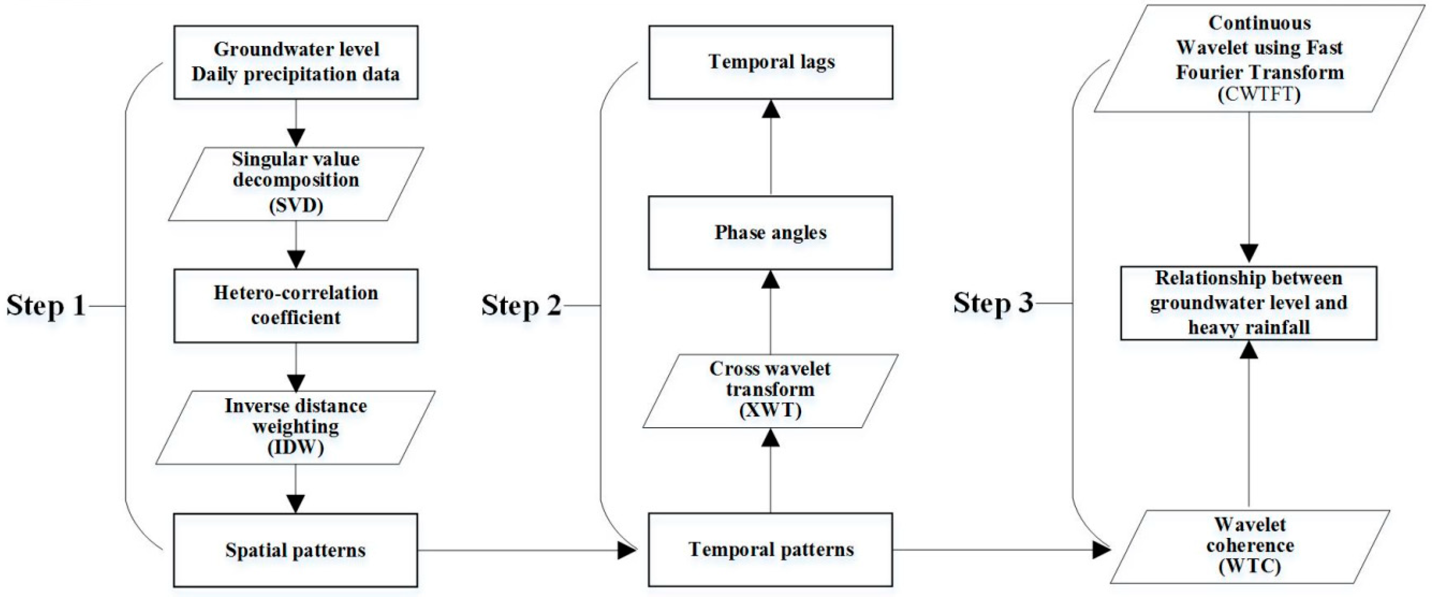
2.3. Singular Value Decomposition

The SVD method was used to identify the spatial modes of the relationship between groundwater level and rainfall for the whole basin, assuming that n is the number of records for a single sample (n = 432 in this study), p is the number of precipitation gauges (p = 45 in this study), q is the number of observation wells (q = 50 in this study). The precipitation data is matrix X_45×432, groundwater data is matrix Y_50×432, and their covariance matrix is A_45×50:

$$A_{p\times q}=\frac{1}{n}XY{}^{\prime }=\frac{1}{n}\left(\begin{array}{cccc}{x}_1{y}_1{}^{\prime }& x_1{y}_2{}^{\prime }& ⋮& x_1{y}_q{}^{\prime }\\ x_2{y}_1{}^{\prime }& x_2{y}_2{}^{\prime }& ⋮& x_2{y}_q{}^{\prime }\\ ⋮& ⋮& ⋮& ⋮\\ x_p{y}_1{}^{\prime }& x_p{y}_2{}^{\prime }& ⋮& x_p{y}_q{}^{\prime }\end{array}\right)$$

(1)

After that, the matrix A_p×q is decomposed into the product of three following matrices:

$$A_{p\times q}=\underset{p\times p}{U} \underset{p\times q}{\mathrm{\Lambda }} \underset{q\times q}{V{}^{\prime }}$$

(2)

where U and V are orthogonal matrices, $U{}^{\prime }U=I$ and $V{}^{\prime }V=I$, and $\mathrm{\Lambda }$ is a diagonal matrix composed of non-negative singular values. Elements of nonzero elements are singular values in the matrix, and its number is s, which is the rank of the matrix. $\lambda$ are eigenvalues of the matrix, which are sorted by size to ${\lambda }_1\ge {\lambda }_2\ge \cdots \ge {\lambda }_q$. The columns of U and V are orthonormal eigenvectors of $AA{}^{\prime }$ and $A{}^{\prime }A$, respectively.

The expansion coefficients of matrix X_45×432 and Y_50×432 can be expressed as:

$$A_{p\times n}=\underset{p\times p}{U{}^{\prime }} \underset{\mathrm{p}\times n}{X}$$

(3)

$$B_{q\times n}=\underset{q\times q}{V{}^{\prime }} \underset{q\times n}{Y}$$

(4)

where $A_{p\times n}$ and $B_{q\times n}$ are the expansion coefficients.

Contribution rate g(k) of the kth modes to square covariance was defined as followed:

$$g\left(k\right)=\frac{{\lambda }_k^2}{{\displaystyle \sum _{i=1}^s{\lambda }_i^2}}$$

(5)

Heterocorrelation coefficient (r) of the kth modes was calculated as followed:

$$r\left(Y,b_k\left(t\right)\right)=\frac{\langle Y\left(t\right)b_t\left(t\right)\rangle }{{\langle Y^2\left(t\right)\rangle }^{1/2}{\langle a_k^2\left(t\right)\rangle }^{1/2}}$$

(6)

where < > is the average operation.

2.4. Spatial Interpolation

In recent years, many spatial interpolation methods have been applied to study the spatial distributions of groundwater and precipitation. The inverse distance weighting method (IDW) gave the lowest mean error among the three common interpolation methods (spline, ordinary kriging, and inverse distance weighting). In addition, the method has been applied widely all over the world [34,35]. Thus, in this study, the IDW method was applied to analyze the spatial variation of each variable using a minimum of three neighbor points and a maximum of five neighbor points, a distance powered to two. Moreover, the interpolation results was validated using the cross-validation method. The spatial interpolation error is 4.2%.

2.5. Cross-Wavelet and Continuous Wavelet Using Fast Fourier Transform

The cross-wavelet was used for demonstrating the temporal association between groundwater level and rainfall. The XWT of the two time series x_n and y_n can be defined as W^XY = W^XW^Y*, where * stands for their complex conjugation. Their cross-wavelet power is defined as |W^XY|. The complex parameter, arg(W^xy), can be considered as the local relative phase between x_n and y_n in time frequency space. The theoretical distribution of the cross-wavelet power and its background power spectra, $p_k^X$ and $p_k^Y$, for two time series can be referenced to Torrence and Compo [22], which is expressed as follows:

$$D\left(\frac{\left|W_n^X\left(s\right)W_n^{Y*}\left(s\right)\right|}{{\sigma }_X{\sigma }_Y}<p\right)=\frac{Z_v\left(p\right)}{v}\sqrt{p_k^X{p}_k^Y}$$

(7)

where Z_v(p) denotes the confidence level associated with the probability p of a probability distribution function which is defined by the square root of the product of two χ² distribution.

The phase difference between the two time series over the basin with a statistical significance above 5% was calculated as follows:

$$a_m=\begin{array}{ccc}\arg \left(X,Y\right)& with& X\end{array}={\displaystyle \sum _{i=1}^n\cos \left(a_i\right)\begin{array}{cc}& and\begin{array}{cc}& Y={\displaystyle \sum _{i=1}^n\sin \left(a_i\right)}\end{array}\end{array}}$$

(8)

where a_m is the circular mean of a set of phase angles (a_i, i = 1, 2, …, n).

The temporal lags (T_lag) were calculated as followed:

$$T_{lag}=1.01a_m$$

(9)

In order to analyze the temporal change of the different components in multiple time scales, the WTC method was applied to identify the intensity of the covariance of two time series, x_n and y_n, in time–frequency domains. Ranging from 0 to 1, where 1 represents the highest covariance between x_n and y_n, the values of the wavelet squared coherency R were calculated as follows [21]:

$$R_n^2\left(s\right)=\frac{{\left|S\left(s^{-1}{W}_n^{xy}\left(s\right)\right)\right|}^2}{S\left(s^{-1}\left|W_n^x{\left(s\right)}^2\right|\right)\cdot S{\left(s^{-1}\left|W_n^y\left(s\right)\right|\right)}^2}$$

(10)

where $W_n^x$ and $W_n^y$ are the wavelet transforms of the time series x and y, respectively, according to time t, and $W_n^{xy}$ is their cross-wavelet spectrum. S represents a smoothing operator and can be expressed as:

$$S\left(W\right)=S_{scale}\left(S_{time}\left(W_n(s)\right)\right)$$

(11)

where S_scale and S_time represent the smoothing along the wavelet scale and time, respectively. For the Morlet wavelet, a suitable smoothing operator is given by Torrence and Webster [22] as follows:

$$S_{time}{\left(W\right)|}_s={\left(W_n\left(s\right)\ast c_1^{-n^2/2s^2}\right)|}_s,{\left(W_n\left(s\right)\ast c_2\prod \left(0.6s\right)\right)|}_n$$

(12)

where c₁ and c₂ are normalized constants and Π is the rectangle function. The factor of 0.6 is the empirically determined scale decorrelation length for the Merlet wavelet [26].

In this study, the wavelet analysis was performed by using the Matlab toolbox developed by Grinsted et al. [21], which is available at http://noc.ac.uk/using-science/crosswavelet-wavelet-coherence.

In addition, original signals of groundwater level and precipitation were decomposed and reconstructed via the continuous wavelet using fast Fourier transform (CWTFT) method, respectively. A more complete process of the methodology was described by Montejo [36]. Furthermore, a conceptual framework of research procedure was shown in Figure 2 to demonstrate the analytical design in this study.

3. Results

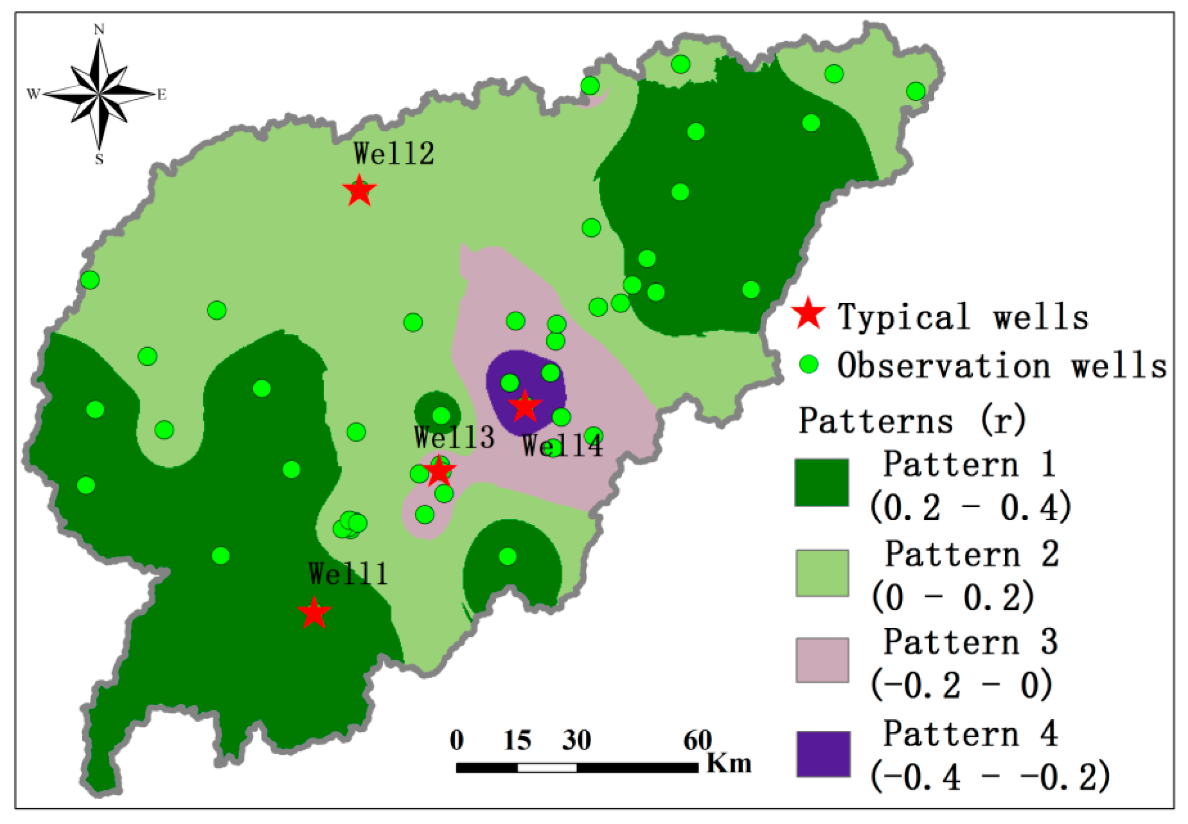
3.1. Spatial Mode Recognition between Groundwater and Precipitation

One major mode has been identified based on the SVD method, which explains 97.1% of the spatial relationship between the five-day groundwater level and precipitation across the Naoli River Basin during 2008–2013. Based on the heterocorrelation coefficient (r) of the major mode, the relationship between groundwater level and precipitation was divided into four spatial patterns in the entire basin (Figure 3). The spatial distribution of r represents the correlation between the expansion coefficient of groundwater level and precipitation in space.

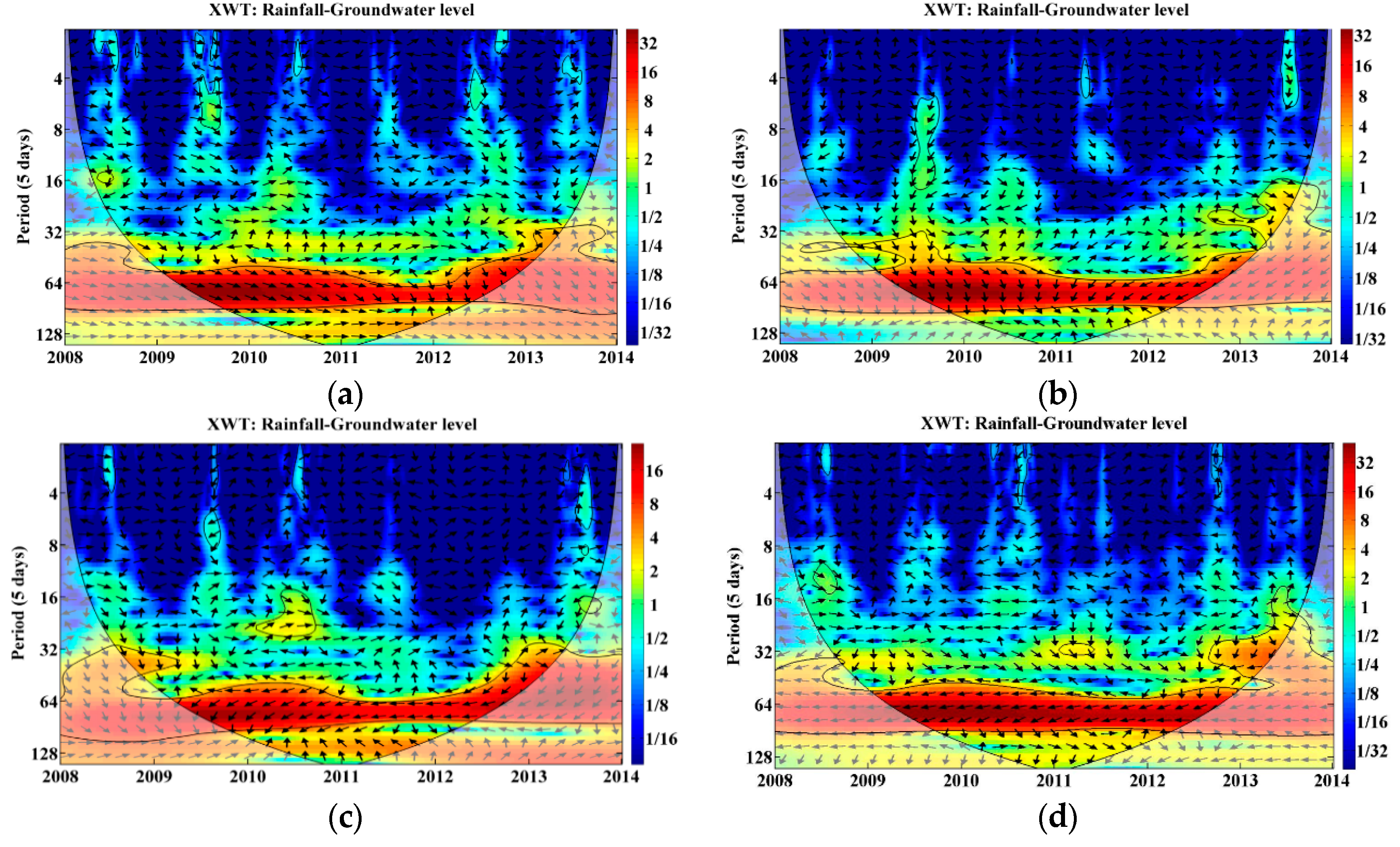
3.2. Temporal Patterns Recognition between Groundwater Level and Precipitation

The typical wells were randomly selected in four pattern regions, and the meteorological stations closest to the typical wells were selected, respectively. The comparisons of the time series between groundwater levels and precipitation during 2008–2013 were shown for four patterns (Figure 4). The groundwater level dynamic is characterized by a periodic change of annual scale in four patterns. In pattern 1 (Figure 4a), the groundwater level is sensitive to changes in precipitation, which quickly increases as precipitation increases, and decreases as precipitation decreases. In pattern 2 (Figure 4b), the sensitivity of groundwater level to precipitation is delayed. When the precipitation occurs, the groundwater level rise will be delayed until after a certain period of time. In pattern 3 (Figure 4c), groundwater level shows a significantly declining trend during 2008–2012. When precipitation occurs, the level rises after a period of time. In pattern 4 (Figure 4d), the dynamic of the groundwater level is significantly delayed by that of precipitation. The groundwater level is in the trough during the wet period and the peak during the dry period of every year.

Based on XWT results, the time–frequency relationships and phase angles between groundwater and precipitation are shown in Figure 5. The dynamic of the groundwater level has a correlation of 5% significance level with that of precipitation for four patterns in a range of 230–480 (46 × 5–96 × 5) days throughout the entire study period, which are the areas surrounded by black lines (Figure 5). This means that there is a response period of 230–480 days for precipitation in groundwater. In addition, there are also some local significant intervals, such as the significant correlation shown with a range of 20–40 (4 × 5–8 × 5) days for pattern 1 in 2009 (Figure 5a), with a range of up to 30 (0 × 5–6 × 5) days for pattern 2 in 2013 (Figure 5b), and so on. These features indicate that precipitation has a strong effect on groundwater level change in these time scales during the entire study period. In other words, the response of groundwater to precipitation is significant in these time scales. In addition, the phase angles had an increasing trend in all patterns during 2008–2013, which means the response time of groundwater level to precipitation for each pattern was increasing.

As with the XWT, the mean phase angle between groundwater level and precipitation was calculated during 2008–2013. Based on the mean phase angle, the temporal lag of variation of groundwater level relative to precipitation in significant regions for four wells was also calculated. That of other wells also was calculated by the same method (

Table 1. Mean phase angles (±std) and temporal lags (±std) over the regions for the four patterns in a period of 365 days.

SVD Patterns	Phase Angles (°)	Temporal Lags (day)
Pattern 1	27 (±8)	27.4 (±8.1)
Pattern 2	106 (±13)	107.5 (±13.2)
Pattern 3	138 (±11)	139.9 (±11.2)
Pattern 4	171 (±20)	173.4 (±20.3)

). In pattern 1, the phase angle between groundwater level and precipitation is the smallest, which is 27° (std: ±8°), and the temporal lag of 27.4 (std: ±8.1) days is also the smallest of the four patterns. In addition, the phase angle of pattern 4, which is 171° (std: ±20°), is the largest of the four patterns. Similarly, the temporal lag of 173.4 (std: ±20.3) days is also the largest of the four patterns.

Except for the relevant time scales mentioned above, more local correlations between groundwater level and heavy rainfall was found based on the WTC method for the four patterns during 2008–2013 (Figure 6). The correlation with a 5% significance level was shown with a range of 0–10 (0 × 5–2 × 5) days in 2008, 40–80 (8 × 5–16 × 5) in 2009, and 15–80 (3 × 5–16 × 5) days in 2012 for pattern 1 (Figure 6a); a range of 20–60 (4 × 5–12 × 5) days in 2008, 20–120 (4 × 5–24 × 5) days in 2009, 30–80 (6 × 5–16 × 5) days in 2011, and 15–30 (3 × 5–6 × 5) days in 2013 for pattern 2 (Figure 6b); a range of 160–240 (32 × 5–48 × 5) days during 2008–2009, 0–25 (0 × 5–5 × 5) days in 2010, 70–90 (14 × 5–18 × 5) days in 2011, and 10–25 (2 × 5–5 × 5) days in 2013 for pattern 3 (Figure 6c); a range of 0–15 (0 × 5–3 × 5) days in 2008, 65–100 (13 × 5–20 × 5) days in 2010, 100–165 (20 × 5–35 × 5) days in 2011, and 50–70 (10 × 5–14 × 5) days in 2013 for t pattern 4 (Figure 6d). These features in the results may be explained by the responses of the groundwater level dynamics to heavy rainfalls.

In summary, the response characteristics of groundwater level to precipitation not only were displayed with the annual time scale throughout the entire study period, but also were exhibited with many local time scales in the Naoli River Basin.

4. Discussion

4.1. The Practical Value of the Method

Previous studies have applied hydrological models to investigate the relationship between groundwater level and precipitation [9,37,38,39,40,41]. However, these models often require large datasets, such as precipitation, groundwater level, runoff, soil type, land use, topography, DEM, lithology, and aquifer parameters, making their applications difficult to many areas without detailed field measurements and historical information. Not only will it take too much time, but also be costly to collect data. Therefore, a simple and economical way should be used for identifying the spatiotemporal response of groundwater level dynamics to precipitation. A novel method is proposed in this study by combining the SVD and cross-wavelet approaches to identify the spatiotemporal relationship between groundwater level and precipitation for the Naoli River Basin in Northeast China. This method can characterize the features of response based on the measured hydrological signals inherent in the observations. Moreover, in this approach, the temporal lags of groundwater level dynamics to precipitation at different regions can be identified [36,42,43,44,45,46]. Therefore, the spatiotemporal patterns of characterized results can help to understand hydrological processes, validate the simulated results of a hydrological model, and promote sustainable use of groundwater resources [10,42,43,44]. In addition, the results can also help assess aquifer vulnerability to climate change [45].

4.2. Factors Influencing the Relationship between Groundwater Level and Precipitation

Based on the method combining SVD and cross-wavelet approaches, four spatiotemporal patterns were identified between groundwater level and precipitation in the Naoli River Basin, Northeast China. In space, there are different temporal lags of groundwater level dynamics to precipitation for the four patterns. The reasons for the finding may be explained by:

(1) Human activities

As mentioned above, land use and land cover in the Naoli River Basin has changed greatly since the 1950s. Almost 80% of wetlands were converted into cultivated land due to rapid economic development [26], of which the sum of the paddy fields occupy 22.7% (or 0.55 × 10⁴ km²). The rice is the main plant in the basin and is the largest water user, especially in the growth period from May to August [46]. In the Naoli River Basin, the main purpose of groundwater pumping is to meet the need of agricultural irrigation [47]. Wu [48] has shown that the groundwater pumping has increased from 0.94 × 10⁸ m³ in 1988 to 28.4 × 10⁸ m³ in 2013 in the Naoli River Basin (Figure 7). In fact, the pumping has become one of the most important drainage ways of groundwater [49,50,51]. The natural balance of the groundwater is affected, and the dynamics of the groundwater change. If the amount of groundwater extracted is equal to that of the groundwater recharge, and the groundwater level is at a lower level than the original average water level, it will experience larger changes, but it will not continue to decline [52]. However, if the amount is too large and exceeds the groundwater recharge, the groundwater level will continue to decline, resulting in an increase of the unsaturated zone’s thickness (Figure 4), which in turn has resulted in an increase of temporal lags in the response of the groundwater level to precipitation (Figure 5). If the overexploration remains unchanged or continues to increase, the response time of the groundwater level to precipitation will increase further. The correlation between the lag time of two factors and the thickness of the unsaturated zone has been studied in previous research works [53,54]. For example, Yang et al. [54] proved by experiments that when the thickness of the unsaturated zone is greater than the limit of the diving evaporation, the infiltration rate decreases with the increase of the unsaturated zone thickness, and then the temporal lags increase. In this study, the phenomenon can also be observed in Figure 4 and Figure 5. For pattern 1, the groundwater depth is shallow as well as less than 5 m (Figure 1d), the groundwater level variation is very highly sensitive to precipitation, and temporal lags were also reduced compared to other patterns. For the other patterns, the groundwater depths were all more than 5 m (Figure 1d), and the temporal lags were also larger than that of pattern 1. In addition, the phase angles were increasing with the increase of the unsaturated zone thickness. This phenomenon demonstrates that the temporal lags were increasing with the increase of the unsaturated zone thickness for the individual pattern (Figure 5). This may be a signal of groundwater depletion due to groundwater pumping for agricultural irrigation [55].

(2) Lithology of the aquifer

Except for the effect of human activities, the lithology of the aquifer is also one of the important factors influencing the relationship between groundwater and precipitation [56,57]. In general, different lithologies of the aquifer have different hydrogeological parameters, that is, the hydraulic conductivity, the recharge coefficient of precipitation infiltration, specific yield, and so on [58,59]. Therefore, the different patterns were shown in space regarding the temporal lags of groundwater level dynamics to precipitation. Previous studies showed that the distribution area of mountainous areas or residual hillocks in the basin belongs to the aquifers of the bedrock fissure, which is also the discharge area of aquifers [31], and the plain area of the basin is the recharge area of the groundwater. In this study, four patterns were identified in the Naoli River Basin. It is worth noting that both the temporal lag and groundwater level variation are all smallest for pattern 1 of all the patterns (Figure 4a). That demonstrates that the groundwater is easily recharged by precipitation and is quickly discharged into rivers through underground runoff in aquifers of the bedrock fissure. Therefore, the response of groundwater to precipitation is more rapid, but there is no obvious change in water level. However, the temporal lag and groundwater level variation are all largest for pattern 4 of all the patterns (Figure 4d), which indicates that when the groundwater is recharged by precipitation, the hydraulic gradient is not obviously increased because it is far away from the discharge area, and the increased intensity of groundwater runoff is not significant, and then the water level rises.

(3) Intensity of precipitation

Precipitation is one of the most important sources for groundwater. Its intensity will have a strong impact on groundwater dynamics [11,60]. However, it is different in the spatiotemporal relationship between groundwater level and precipitation, because of the influence of the factors mentioned above. In addition, it is worth noting that the groundwater level dynamics are very sensitive to extreme rainfall in the Naoli River Basin (Figure 4 and Figure 6).

In order to clearly reveal the relationship between the groundwater level and heavy rainfall, signals of groundwater level and precipitation were reconstructed based on the CWTFT method, respectively (Figure 8). These reconstructed signals mean the intensity of groundwater level or precipitation change per unit of time. In pattern 1, the amplitude of groundwater level is highly consistent with that of precipitation (Figure 8a). In other patterns, the amplitudes of groundwater levels are relatively gentle (Figure 8b,c), which have weakly responded to levels of precipitation. However, some strong amplitudes are identified during April and May in every year in pattern 4, which may be explained by the fact that groundwater is pumped for the irrigation of paddy fields, resulting in a sharp drop in groundwater levels [28]. This result has been demonstrated by some previous studies [27,46,61,62,63]. In addition, in order to cope with droughts and floods, the recharge of heavy rainfall on groundwater and the interannual allocation of water resources in underground reservoirs should be carefully studied.

4.3. Uncertainties of This Study

Some uncertainty may exist in identifying the spatiotemporal patterns by combining the SVD and cross-wavelet approaches, because the accuracy of identification may be greatly influenced by the spatial distribution of observation wells and scarcity of measured precipitation data. In addition, accurate spatial and temporal characterization of groundwater recharge can be difficult, due to its dependence on a multitude of physical factors such as land use and hydrogeological heterogeneity, groundwater pumping, and so on [64,65]. Despite the uncertainties and limitations, this method still sheds some light on an understanding of the spatiotemporal response of groundwater level dynamics to precipitation in some regions lacking basic data. Moreover, future studies are needed to constrain the uncertainties and refine the response of groundwater level dynamics to different intensities of precipitation.

5. Conclusions

This study identified the spatiotemporal responses of the groundwater table to precipitation in the Naoli River Basin, Northeast China, using a method combining SVD and cross-wavelet approaches. Based on the findings, the following conclusions can be drawn:

(1)

The new method can be a cost-effective approach for identifying the spatiotemporal responses of the groundwater table to precipitation, especially in areas where hydrological models are difficult to construct due to a lack of basic data.

(2)

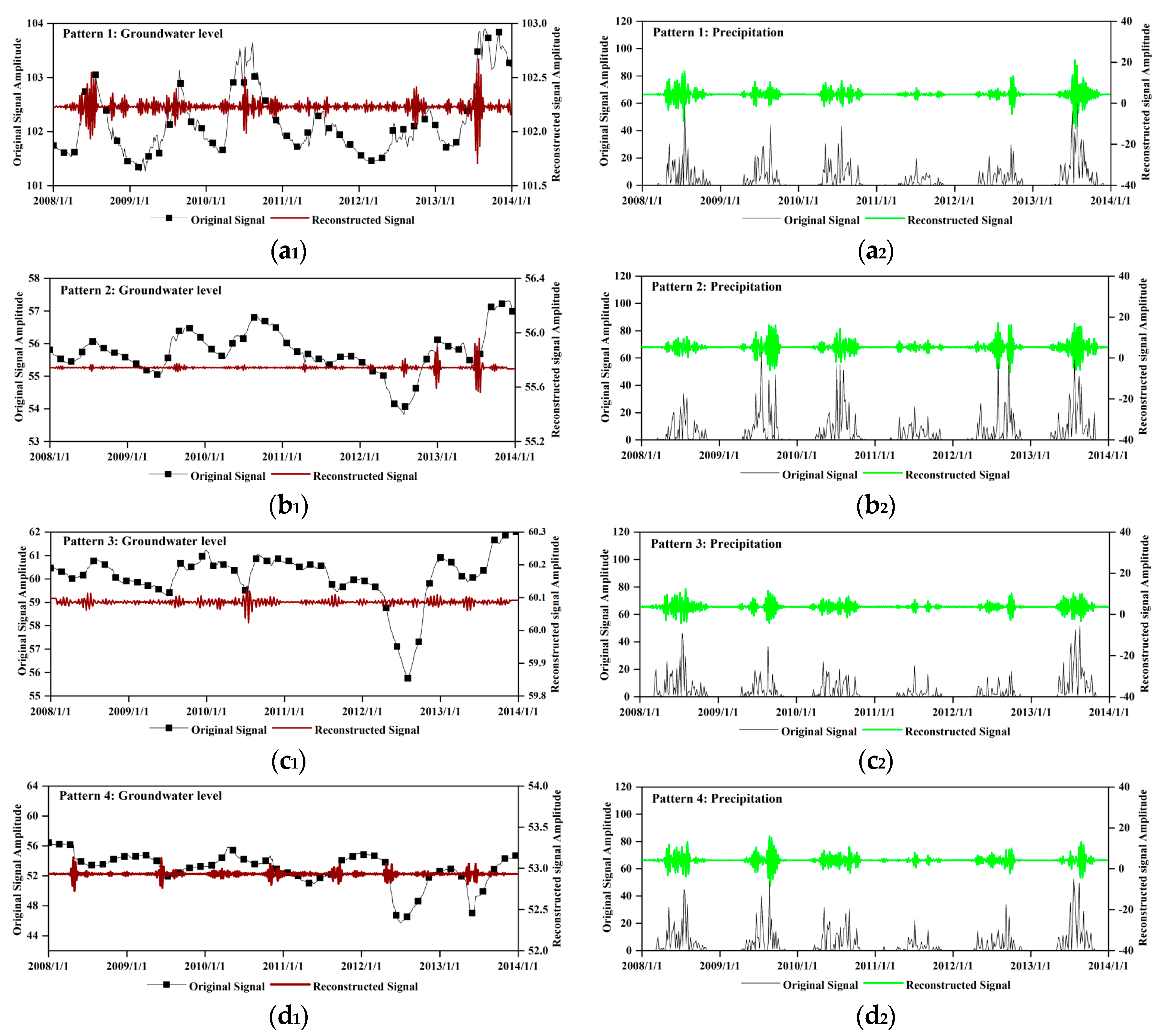
The major mode of the relation between groundwater and precipitation was divided into four patterns in the Naoli River Basin. In general, the lag time is 27.4 (std: ±8.1) days, 107.5 (std: ±13.2) days, 139.9 (std: ±11.2) days, and 173.4 (std: ±20.3) days for the patterns 1–4, respectively.

(3)

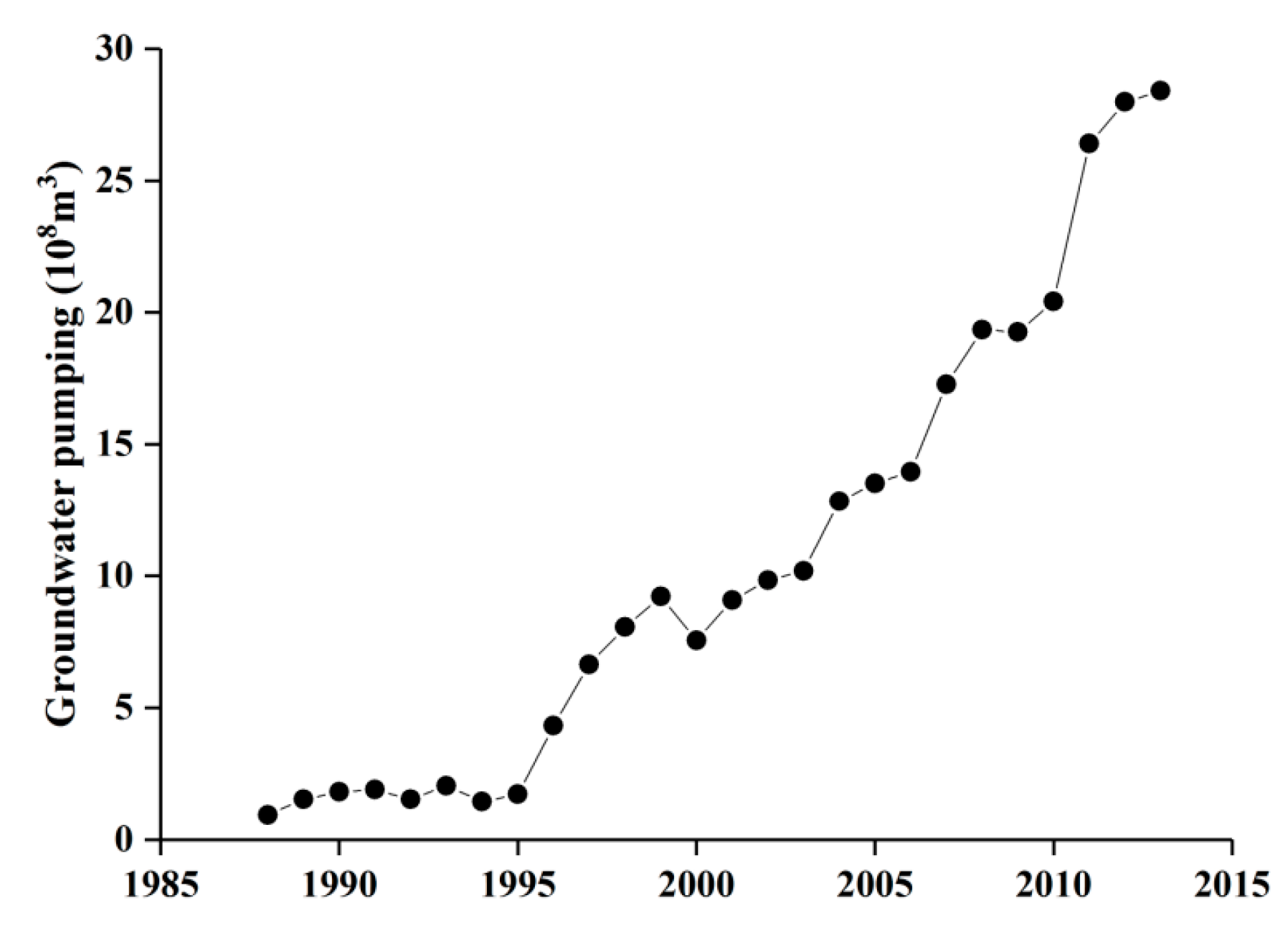
The rapid agricultural development relying on groundwater irrigation has led to an increase of the unsaturated zone thickness, which in turn results in an increase of temporal lags in the groundwater table response to precipitation.

(4)

The response of the groundwater table in the studied river basin is very sensitive to heavy rainfall. Thus, enhancing the utilization of the heavy rainfall and flood resources by groundwater may be an effective way to recharge the groundwater. Furthermore, it is possible to make use of the interannual allocation of water resources for the groundwater reservoir to deal with extreme hydrological events of flood and drought.

References

1. Siebert, S.; Burke, J.; Faures, J.-M.; Frenken, K.; Hoogeveen, J.; Döll, P.; Portmann, F.T. Groundwater use for irrigation–a global inventory. Hydrol. Earth Syst. Sci. 2010, 14, 1863–1880. [Google Scholar] [CrossRef] [Green Version]
2. Alley, W.M.; Healy, R.W.; LaBaugh, J.W.; Reilly, T.E. Flow and storage in groundwater systems. Science 2002, 296, 1985–1990. [Google Scholar] [CrossRef] [PubMed]
3. Konikow, L.F.; Kendy, E. Groundwater depletion: A global problem. Hydrogeol. J. 2005, 13, 317–320. [Google Scholar] [CrossRef]
4. Asoka, A.; Gleeson, T.; Wada, Y.; Mishra, V. Relative contribution of monsoon precipitation and pumping to changes in groundwater storage in India. Nat. Geosci. 2017, 10, 109–117. [Google Scholar] [CrossRef]
5. Scanlon, B.R.; Longuevergne, L.; Long, D. Ground referencing GRACE satellite estimates of groundwater storage changes in the California Central Valley, USA. Water Resour. Res. 2012, 48. [Google Scholar] [CrossRef] [Green Version]
6. Hughes, J.; Petrone, K.; Silberstein, R. Drought, groundwater storage and stream flow decline in southwestern Australia. Geophys. Res. Lett. 2012, 39, 34–42. [Google Scholar] [CrossRef]
7. MacDonald, A.M.; Bonsor, H.C.; Dochartaigh, B.É.Ó.; Taylor, R.G. Quantitative maps of groundwater resources in Africa. Environ. Res. Lett. 2012, 7, 024009. [Google Scholar] [CrossRef]
8. Feng, W.; Zhong, M.; Lemoine, J.M.; Biancale, R.; Hsu, H.T.; Xia, J. Evaluation of groundwater depletion in North China using the Gravity Recovery and Climate Experiment (GRACE) data and ground-based measurements. Water Resour. Res. 2013, 49, 2110–2118. [Google Scholar] [CrossRef]
9. Zhang, X.; Ren, L.; Kong, X. Estimating spatiotemporal variability and sustainability of shallow groundwater in a well-irrigated plain of the Haihe River basin using SWAT model. J. Hydrol. 2016, 541, 1221–1240. [Google Scholar] [CrossRef]
10. Yu, H.-L.; Lin, Y.-C. Analysis of space–time non-stationary patterns of rainfall–groundwater interactions by integrating empirical orthogonal function and cross wavelet transform methods. J. Hydrol. 2015, 525, 585–597. [Google Scholar] [CrossRef]
11. Owor, M.; Taylor, R.G.; Tindimugaya, C.; Mwesigwa, D.; Bovolo, C.I.; Parkin, G.; Sophocleous, M. Rainfall intensity and groundwater recharge: Empirical evidence from the Upper Nile Basin. Environ. Res. Lett. 2009, 4, 035009. [Google Scholar] [CrossRef]
12. Dhakal, A.S.; Sullivan, K. Shallow groundwater response to rainfall on a forested headwater catchment in northern coastal California: Implications of topography, rainfall, and throughfall intensities on peak pressure head generation. Hydrol. Process. 2014, 28, 446–463. [Google Scholar] [CrossRef]
13. Tsai, J.-P.; Chang, L.-C.; Chang, P.-Y.; Lin, Y.-C.; Chen, Y.-C.; Wu, M.-T.; Yu, H.-L. Spatial-temporal pattern recognition of groundwater head variations for recharge zone identification. J. Hydrol. 2017, 549, 351–362. [Google Scholar] [CrossRef]
14. Wang, B.; Lee, J.-Y.; Xiang, B. Asian summer monsoon rainfall predictability: A predictable mode analysis. Clim. Dyn. 2015, 44, 61. [Google Scholar] [CrossRef]
15. Cao, J.; Yao, P.; Wang, L.; Liu, K. Summer rainfall variability in low-latitude highlands of China and subtropical Indian Ocean dipole. J. Clim. 2014, 27, 880–892. [Google Scholar] [CrossRef]
16. Omondi, P.; Ogallo, L.A.; Anyah, R.; Muthama, J.M.; Ininda, J. Linkages between global sea surface temperatures and decadal rainfall variability over Eastern Africa region. Int. J. Climatol. 2013, 33, 2082–2104. [Google Scholar] [CrossRef]
17. Lau, K.M.; Wu, H.T. Principal Modes of Rainfall-SST Variability of the Asian Summer Monsoon: A Reassessment of the Monsoon-ENSO Relationship. J. Clim. 2000, 14, 2880–2895. [Google Scholar] [CrossRef]
18. Wallace, J.M.; Smith, C.; Bretherton, C.S. Singular value decomposition of wintertime sea surface temperature and 500-mb height anomalies. J. Clim. 1992, 5, 561–576. [Google Scholar] [CrossRef]
19. Rauniyar, S.P.; Kevin, J.; Walsh, E. Spatial and temporal variations in rainfall over Darwin and its vicinity during different large-scale environments. Clim. Dyn. 2016, 46, 671. [Google Scholar] [CrossRef]
20. Bretherton, C.S.; Smith, C.; Wallace, J.M. An intercomparison of methods for finding coupled patterns in climate data. J. Clim. 1992, 5, 541–560. [Google Scholar] [CrossRef]
21. Grinsted, A.; Moore, J.C.; Jevrejeva, S. Application of the cross wavelet transform and wavelet coherence to geophysical time series. Nonlinear Process. Geophys. 2004, 11, 561–566. [Google Scholar] [CrossRef]
22. Torrence, C.; Compo, G.P. A practical guide to wavelet analysis. Bull. Am. Meteorol. Soc. 1998, 79, 61–78. [Google Scholar] [CrossRef]
23. Huang, S.; Li, P.; Huang, Q.; Leng, G.; Hou, B.; Ma, L. The propagation from meteorological to hydrological drought and its potential influence factors. J. Hydrol. 2017, 547, 184–195. [Google Scholar] [CrossRef]
24. Huang, S.Z.; Huang, Q.; Chang, J.X.; Leng, G.Y. Linkages between hydrological drought, climate indices and human activities: a case study in the Columbia River basin. Int. J. Climatol. 2016, 36, 280–290. [Google Scholar] [CrossRef]
25. Tan, X.; Gan, T.Y.; Shao, D. Wavelet analysis of precipitation extremes over Canadian ecoregions and teleconnections to large-scale climate anomalies. J. Geophys. Res. Atmos. 2016, 121. [Google Scholar] [CrossRef]
26. Dan, W.; Wei, H.; Zhang, S.; Kun, B.; Bao, X.; Yi, W.; Yue, L. Processes and prediction of land use/land cover changes (LUCC) driven by farm construction: The case of Naoli River Basin in Sanjiang Plain. Environ. Earth Sci. 2015, 73, 4841–4851. [Google Scholar] [CrossRef]
27. Wang, X.; Zhang, G.; Xu, Y.J. Impacts of the 2013 Extreme Flood in Northeast China on Regional Groundwater Depth and Quality. Water 2015, 7, 4575–4592. [Google Scholar] [CrossRef]
28. Wang, X.; Zhang, G.; Xu, Y.J. Spatiotemporal groundwater recharge estimation for the largest rice production region in Sanjiang Plain, Northeast China. J. Water Supply Res. Technol.-Aqua 2014, 63, 630–641. [Google Scholar] [CrossRef]
29. Yang, X.; Yang, W.; Zhang, F.; Chu, Y.; Wang, Y.; Yi, X.; Zhang, B.; Guo, H.; Sun, Y. Investigation and Assessment of Groundwater Resources Potential and Eco-Environment Geology in Sanjiang Plain; Geological Publishing House: Beijing, China, 2008. [Google Scholar]
30. Lu, W.; Li, P.; Wang, F.; Guo, L. Three-Dimensional Numerical Simulation of Groundwater in Naolihe Watershed. J. Jilin Univ. (Earth Sci. Ed.) 2007, 37, 541–545. [Google Scholar]
31. Wu, C. Analysis Groundwater Resources Volume of Naoli River Basin. Syst. Sci. Compr. Stud. Agric. 2011, 4, 385–389. [Google Scholar]
32. Wang, X.; Zhang, G.; Xu, Y.J.; Shan, X. Defining an Ecologically Ideal Shallow Groundwater Depth for Regional Sustainable Management: Conceptual Development and Case Study on the Sanjiang Plain, Northeast China. Water 2015, 7, 3997–4025. [Google Scholar] [CrossRef]
33. Meng, X.-Y.; Wang, H.; Cai, S.-Y.; Zhang, X.-S.; Leng, G.-Y.; Lei, X.-H.; Shi, C.-X.; Liu, S.-Y.; Shang, Y. The China Meteorological Assimilation Driving Datasets for the SWAT Model (CMADS) Application in China: A Case Study in Heihe River Basin. Prepints 2016. [Google Scholar] [CrossRef]
34. Nam, W.-H.; Hong, E.-M.; Choi, J.-Y. Has climate change already affected the spatial distribution and temporal trends of reference evapotranspiration in South Korea? Agric. Water Manag. 2015, 150, 129–138. [Google Scholar] [CrossRef]
35. Raziei, T.; Pereira, L.S. Spatial variability analysis of reference evapotranspiration in Iran utilizing fine resolution gridded datasets. Agric. Water Manag. 2013, 126, 104–118. [Google Scholar] [CrossRef]
36. Montejo, L.A.; Suarez, L.E. An improved CWT-based algorithm for the generation of spectrum-compatible records. Int. J. Adv. Struct. Eng. 2013, 5, 26. [Google Scholar] [CrossRef]
37. Chung, I.-M.; Kim, N.-W.; Lee, J.; Sophocleous, M. Assessing distributed groundwater recharge rate using integrated surface water-groundwater modelling: Application to Mihocheon watershed, South Korea. Hydrogeol. J. 2010, 18, 1253–1264. [Google Scholar] [CrossRef]
38. Liu, H.-L.; Chen, X.; Bao, A.-M.; Wang, L. Investigation of groundwater response to overland flow and topography using a coupled MIKE SHE/MIKE 11 modeling system for an arid watershed. J. Hydrol. 2007, 347, 448–459. [Google Scholar] [CrossRef]
39. Wheater, H. Hydrological processes, groundwater recharge and surface-water/groundwater interactions in arid and semi-arid areas. In Groundwater Modeling in Arid and Semi-Arid Areas; Cambridge University Press: Cambridge, UK, 2010; pp. 5–37. [Google Scholar]
40. Wang, L.; Jackson, C.R.; Pachocka, M.; Kingdon, A. A seamlessly coupled GIS and distributed groundwater flow model. Environ. Model. Softw. 2016, 82, 1–6. [Google Scholar] [CrossRef] [Green Version]
41. Hong, N.; Hama, T.; Suenaga, Y.; Aqili, S.W.; Huang, X.; Wei, Q.; Kawagoshi, Y. Application of a modified conceptual rainfall–runoff model to simulation of groundwater level in an undefined watershed. Sci. Total Environ. 2016, 541, 383–390. [Google Scholar] [CrossRef] [PubMed]
42. Kang, S.; Lin, H. Wavelet analysis of hydrological and water quality signals in an agricultural watershed. J. Hydrol. 2007, 338, 1–14. [Google Scholar] [CrossRef]
43. Hsiao, C.-T.; Chang, L.-C.; Tsai, J.-P.; Chen, Y.-C. Features of spatiotemporal groundwater head variation using independent component analysis. J. Hydrol. 2017, 547, 623–637. [Google Scholar] [CrossRef]
44. Lee, C.-H.; Yeh, H.-F.; Chen, J.-F. Estimation of groundwater recharge using the soil moisture budget method and the base-flow model. Environ. Geol. 2008, 54, 1787–1797. [Google Scholar] [CrossRef]
45. Russo, T.A.; Lall, U. Depletion and response of deep groundwater to climate-induced pumping variability. Nat. Geosci. 2017, 10, 105–108. [Google Scholar] [CrossRef]
46. Liu, Y.; Jiang, X.; Zhang, G.; Xu, Y.J.; Wang, X.; Qi, P. Assessment of Shallow Groundwater Recharge from Extreme Rainfalls in the Sanjiang Plain, Northeast China. Water 2016, 8, 440. [Google Scholar] [CrossRef]
47. Liu, D.; Zhang, J.; Fu, Q. Study on complexity of groundwater depth series in well irrigation area of sanjiang plain based on continuous wavelet transform and fractal theory. Res. Soil Water Conserv. 2011, 2, 027. [Google Scholar]
48. Wu, C. Prediction research on groundwater exploitation in Naolihe River basin based on Elman wavelet neural network. J. Water Resour. Water Eng. 2011, 22, 29–35. [Google Scholar]
49. Ruud, N.; Harter, T.; Naugle, A. Estimation of groundwater pumping as closure to the water balance of a semi-arid, irrigated agricultural basin. J. Hydrol. 2004, 297, 51–73. [Google Scholar] [CrossRef]
50. Wada, Y. Impacts of groundwater pumping on regional and global water resources. Terr. Water Cycle Clim. Chang. Nat. Hum.-Induc. Impacts 2016, 71–101. [Google Scholar] [CrossRef]
51. Massuel, S.; Amichi, F.; Ameur, F.; Calvez, R.; Jenhaoui, Z.; Bouarfa, S.; Kuper, M.; Habaieb, H.; Hartani, T.; Hammani, A. Considering groundwater use to improve the assessment of groundwater pumping for irrigation in North Africa. Hydrogeol. J. 2017, 25, 1565–1577. [Google Scholar] [CrossRef]
52. Zhang, R.; Liang, X.; Jin, M.; Wan, L.; Yu, Q. Fundamentals of Hydrogeology, 6th ed.; Geological Press: Beijing, China, 2010. [Google Scholar]
53. Lee, L.; Lawrence, D.; Price, M. Analysis of water-level response to rainfall and implications for recharge pathways in the Chalk aquifer, SE England. J. Hydrol. 2006, 330, 604–620. [Google Scholar] [CrossRef]
54. Zhang, G.; Fei, Y.; Shen, J.; Yang, L. Influence of unsaturated zone thickness on precipitation infiltration for recharge of groundwater. J. Hydraul. Eng. 2007, 38, 611–617. [Google Scholar]
55. Ho, M.; Parthasarathy, V.; Etienne, E.; Russo, T.; Devineni, N.; Lall, U. America’s water: Agricultural water demands and the response of groundwater. Geophys. Res. Lett. 2016, 43, 7546–7555. [Google Scholar] [CrossRef]
56. Helena, B.; Pardo, R.; Vega, M.; Barrado, E.; Fernandez, J.M.; Fernandez, L. Temporal evolution of groundwater composition in an alluvial aquifer (Pisuerga River, Spain) by principal component analysis. Water Res. 2000, 34, 807–816. [Google Scholar] [CrossRef]
57. Chen, Z.; Grasby, S.E.; Osadetz, K.G. Predicting average annual groundwater levels from climatic variables: An empirical model. J. Hydrol. 2002, 260, 102–117. [Google Scholar] [CrossRef]
58. Hatch, C.E.; Fisher, A.T.; Ruehl, C.R.; Stemler, G. Spatial and temporal variations in streambed hydraulic conductivity quantified with time-series thermal methods. J. Hydrol. 2010, 389, 276–288. [Google Scholar] [CrossRef]
59. Gómez-Hernández, J.J.; Gorelick, S.M. Effective groundwater model parameter values: Influence of spatial variability of hydraulic conductivity, leakance, and recharge. Water Resour. Res. 1989, 25, 405–419. [Google Scholar] [CrossRef]
60. Wang, H.; Gao, J.E.; Zhang, M.-J.; Li, X.-H.; Zhang, S.-L.; Jia, L.-Z. Effects of rainfall intensity on groundwater recharge based on simulated rainfall experiments and a groundwater flow model. Catena 2015, 127, 80–91. [Google Scholar] [CrossRef]
61. Zhang, G.; Fei, Y.; Tian, Y.; Wang, Q.; Yan, M. Characteristics of alleviating the over-exploitation and its recharge on the rainstorm flood to the shallow groundwater in the southern plain of Haihe River basin. J. Hydraul. Eng. 2015, 46, 594–601. [Google Scholar]
62. Hartmann, A.; Mudarra, M.; Andreo, B.; Marín, A.; Wagener, T.; Lange, J. Modeling spatiotemporal impacts of hydroclimatic extremes on groundwater recharge at a Mediterranean karst aquifer. Water Resour. Res. 2014, 50, 6507–6521. [Google Scholar] [CrossRef]
63. Taylor, R.G.; Todd, M.C.; Kongola, L. Evidence of the dependence of groundwater resources on extreme rainfall in East Africa. Nat. Clim. Chang. 2013, 3, 374–378. [Google Scholar] [CrossRef] [Green Version]
64. Lerner, D.N.; Issar, A.S.; Simmers, I. Groundwater Recharge: A Guide to Understanding and Estimating Natural Recharge; Heise Hannover: Hannover, Germany, 1990; Volume 8. [Google Scholar]
65. Jyrkama, M.I.; Sykes, J.F. The impact of climate change on spatially varying groundwater recharge in the grand river watershed (Ontario). J. Hydrol. 2007, 338, 237–250. [Google Scholar] [CrossRef]
Figure 1. (a) Geographical locations of the observational wells and precipitation gauge stations used in this study; (b) Land use and land cover (LULC); (c) hydraulic conductivities; and (d) average unsaturated zone thickness in the Naoli River basin, Northeast China.
Water 10 00598 g001
Figure 2. Conceptual framework of the research procedures conducted in this study.
Water 10 00598 g002
Figure 3. Spatial mode between groundwater and precipitation in the Naoli River Basin, Northeast China, based on the SVD method.
Water 10 00598 g003
Figure 4. The time series of groundwater levels and precipitation in the Naoli River Basin, Northeast China, for pattern 1 (a); pattern 2 (b); pattern 3 (c) and pattern 4 (d) during 2008–2013.
Water 10 00598 g004
Figure 5. The cross-wavelet transform (XWT) between precipitation and groundwater in the Naoli River Basin, Northeast China, for pattern 1 (a), pattern 2 (b), pattern 3 (c), and pattern 4 (d), respectively. The significant level of 5% for red noise is displayed as a thick contour, and the relative relationship of phase is denoted as arrows (with anti-phase pointing left, in-phase pointing right).
Water 10 00598 g005
Figure 6. The wavelet coherence (WTC) between precipitation and groundwater in the Naoli River Basin, Northeast China, for pattern 1 (a); pattern 2 (b); pattern 3 (c); and pattern 4 (d), respectively. The significant level of 5% for red noise is displayed as a thick contour, and the relative relationship of phase is denoted as arrows (with anti-phase pointing left, in-phase pointing right).
Water 10 00598 g006aWater 10 00598 g006b
Figure 7. Groundwater pumping during 1988–2013 in the Naoli River Basin, Northeast China.
Water 10 00598 g007
Figure 8. Reconstruction of original signals between groundwater level and precipitation in the Naoli River Basin, Northeast China, during 2008–2013, based on the continuous wavelet using fast Fourier transform (CWTFT) method for pattern 1 (a); pattern 2 (b); pattern 3 (c); and pattern 4 (d), respectively.
Water 10 00598 g008