Experimental and Numerical Modelling of Bottom Intake Racks with Circular Bars


Civil Engineering Department, Universidad Politécnica de Cartagena, Paseo Alfonso XIII, 52, 30203 Cartagena, Spain
*
Author to whom correspondence should be addressed.
Water 2018, 10(5), 605; https://doi.org/10.3390/w10050605
Submission received: 12 March 2018
/
Revised: 2 May 2018
/
Accepted: 3 May 2018
/
Published: 6 May 2018
(This article belongs to the Section Hydraulics and Hydrodynamics)
Abstract
:Bottom rack intake systems are one of the most popular structures for diverting water in steep rivers. Intake systems may be used in ephemeral rivers beds to capture part of the runoff flow in the rainy season. Their behavior has mainly been studied in the laboratory. Nevertheless, it is not possible to analyze the whole problem of characterization with traditional methodologies due to the many effects that occur on the bars. Computational fluid dynamics simulations have been considered as a complement to improve the knowledge of the hydraulic phenomenon. However, the geometry of circular racks may be a challenge due to its complexity. After the validation procedure, the numerical models appear to be a good tool to design intake systems. No remarkable differences were obtained between the three two-equation turbulence models tested. The results show differences of less than 1% in flow profile over the rack. Fit curves have been proposed to estimate the flow profile over the rack with r2 > 95%. Expressions to calculate the discharge coefficient and the collected water through the rack in the clear water case have been proposed and show a good agreement with the laboratory data.
1. Introduction
Intake systems commonly consist of a rack located in the bottom of the channel, so that the water collected passes through the rack. These structures are adopted in small mountain rivers with steep slopes and an irregular riverbed, intense sediment transport, and flash floods. Their design needs to satisfy two primary objectives: to derive as much water as possible and with the minimum quantity of solids.
The behavior of the racks system varies as a function of different factors, such as: the size of the bars, their shape, the void ratio (spacing between bars), the longitudinal slope, and the incoming flow conditions.
Authors often assume some simplifications in the analysis of clear water flows: the flux over the rack is considered one-dimensional, the flow decreases progressively, or the hydrostatic pressure distribution acts over the rack in the flow direction. Regarding the simplification of the energy head over the rack, there are two considerations: horizontal energy level and energy level parallel to the rack plane (Table 1).
The discharge coefficient in bottom intake racks changes along the wetted rack length and depends on the shape of the bars (Righetti et al. [1]). The space between bars also influences the flow derived along the racks (Brunella et al. [2]). The distribution of the discharge coefficient along the rack may be related to the pressure field of flow in the slit of the bars (Castillo et al. [3]).
All these issues make it important to determine the discharge coefficient along racks in bottom intake systems. The classical approaches of intake racks consider a two-dimensional perspective in the vertical plane of the rack. However, upon analyzing the flow near the bars, that flow becomes extremely three-dimensional, rendering the two-dimensional analysis tools less useful. In those cases, the computational fluid dynamics (CFD) models, once they have been validated against experimental values, may help to obtain a better understanding of the phenomenon (Bombardelli [18]; Blocken & Gualtieri [19]). However, numerical models have not been extensively used in this topic (Zerihun [20]; Hosseini et al. [21]; Carrillo et al. [22]).
In numerical modelling, different simplifications have been used. Some authors considered one-dimensional and two-dimensional models to study the hydraulic behavior of rivers and sediment transport phenomena. Nevertheless, flows occurring in hydraulic structures tend to be highly three-dimensional (Bombardelli [18]; Castillo & Carrillo [23]). For this reason, three-dimensional models were considered.
In previous works, the discharge coefficient along the wetted length of rack was experimentally measured and numerically simulated by ANSYS CFX in the case of T-shaped bars (García [10]; Carrillo et al. [22]).
The present work shows experimental measurements and three-dimensional simulations in a bottom intake with racks made with circular bars, considering clear water flow. The values along the rack are compared with previous results with flat bars.
1.1. Wetted Rack Length
There are several proposals to calculate the theoretical wetted rack length L necessary to derive a defined flow rate q1. The required length may differ by up to double in some cases, depending on the author (García [10]). This is due to the variation of the experimental conditions used to adjust the discharge coefficient, such as the shape of the bars, their separation and width, the void ratio, the approximation flow conditions, the initial flow depth h1, or the longitudinal rack slope θ (Castillo et al. [24]).
Besides this, the theoretical longitudinal rack slope, θ, has been considered in different ways. Some authors consider the influence of the slope (Garot [25]; Orth et al. [26]; White et al. [27]; Righetti & Lanzoni [9]). However, other researchers experimentally found that there is no further influence for slopes greater than 19º (≈34%) (Brunella et al. [2]).
To avoid rack occlusion, several authors proposed design recommendations from prototype observations in mountain rivers (e.g., Orth et al. [26]; Ract-Madoux et al. [28]; Krochin [17]; Drobir [29]; Bouvard [30]; Raudkivi [31]). From experimental measurements in a flow with coarse sediments, the optimum rack slope to avoid occlusion of the space between bars is in the range of 30–36% (Castillo et al. [3,32]; Bina & Shagi [33]).
1.2. Discharge Coefficient
The orifice equation may be used to calculate the specific derived flow q through the bottom rack per unit of length x and width, qd = dq/dx (m3/s/m). As the collected flow through the rack plane is influenced by the velocity distribution close to it, the velocity coefficient, Cv, considers the deviation from the uniform distribution. In a similar way, as there is a change in the available section, which involves the flow contraction, a contraction coefficient, Cc, may be considered. Both coefficients require experimental measurement and depend on the shape of the bars and the spacing between them. The orifice equation as a function of the total energy available referred to the plane of the rack has been considered by several authors (De Marchi [34]; Motskow [15]; Nakagawa [35]; Krochin [17]; Ahmad & Mittal [36]; Ghosh & Ahmad [37]; Righetti & Lanzoni [9]; Kumar et al. [38]). The general expression may be written as:
where m is the void ratio (relation between the void area and the total area), H the total energy available referred to the plane of the rack, and CqH the discharge coefficient depending on the energy head (CqH = CcCv).
The specific derived flow may also be obtained as a function of the water depth along the rack, h (Garot [25]; Bouvard & Kuntzmann [4]; Noseda [12,13]; Frank [5]; Brunella et al. [2]). Hence, the orifice equation is:
where Cqh is the discharge coefficient as a function of the water depth normal to the rack plane.
Righetti et al. [1] considered that the differential flow of the water collected may be calculated with the following formula:
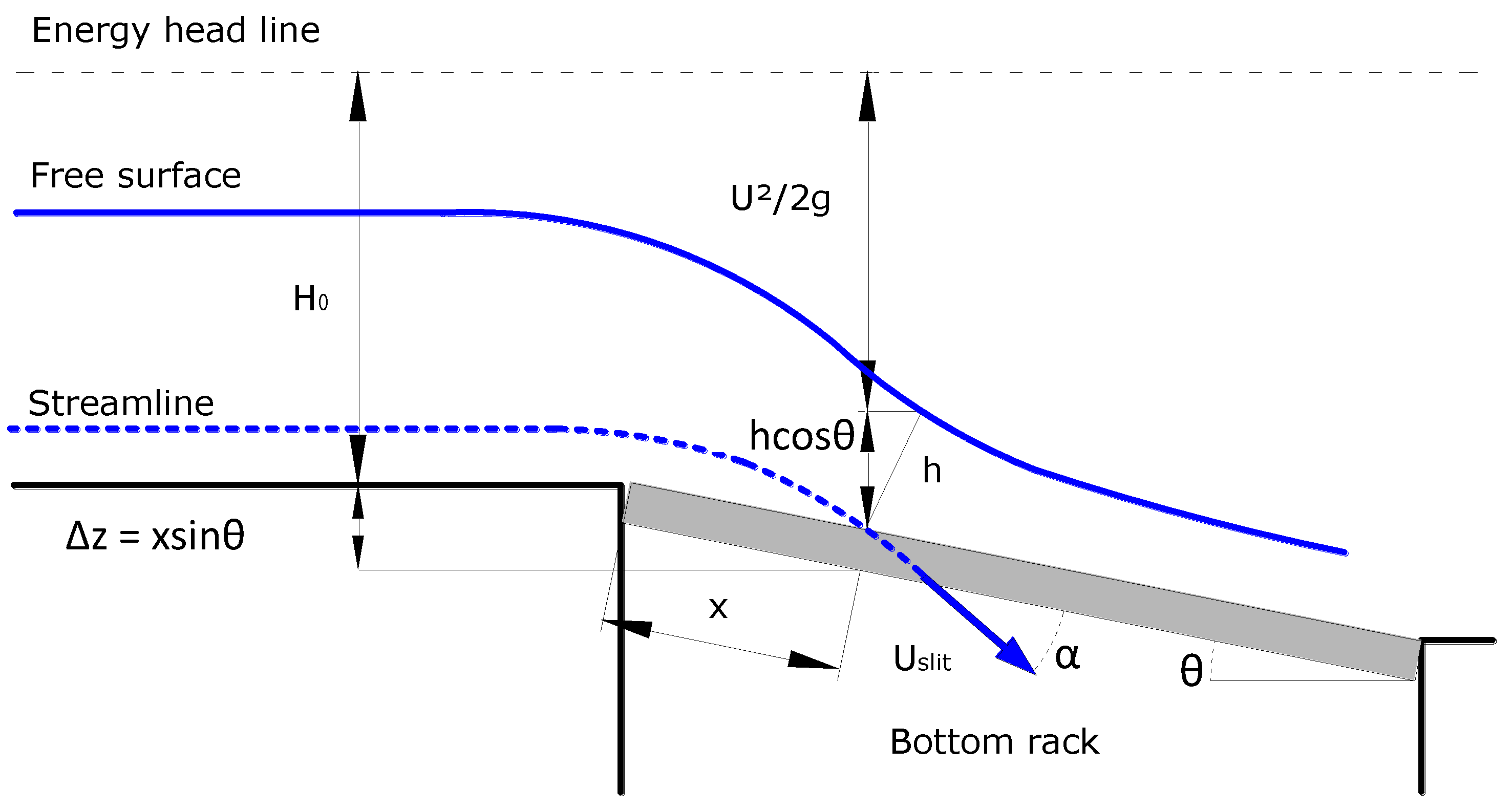
where H0 is the specific energy at the beginning of the rack, and Δz the vertical difference between the initial rack section and the analyzed section.
1.3. Discharge Coefficient
The flow profile over the rack has been analyzed by several authors (Garot [25]; De Marchi [34]; Noseda [12]; Frank [5]; Dagan [16]; García [10]).
Considering velocity measurements in the free surface, Brunella et al. [2] obtained that the dissipation effects are insignificant. However, in the final part of the racks these effects cannot be neglected since the local effects generate friction effects. Differences between measured and calculated depth profiles at the beginning of the rack are due to the consideration of hydrostatic pressure distribution.
2. Physical Device
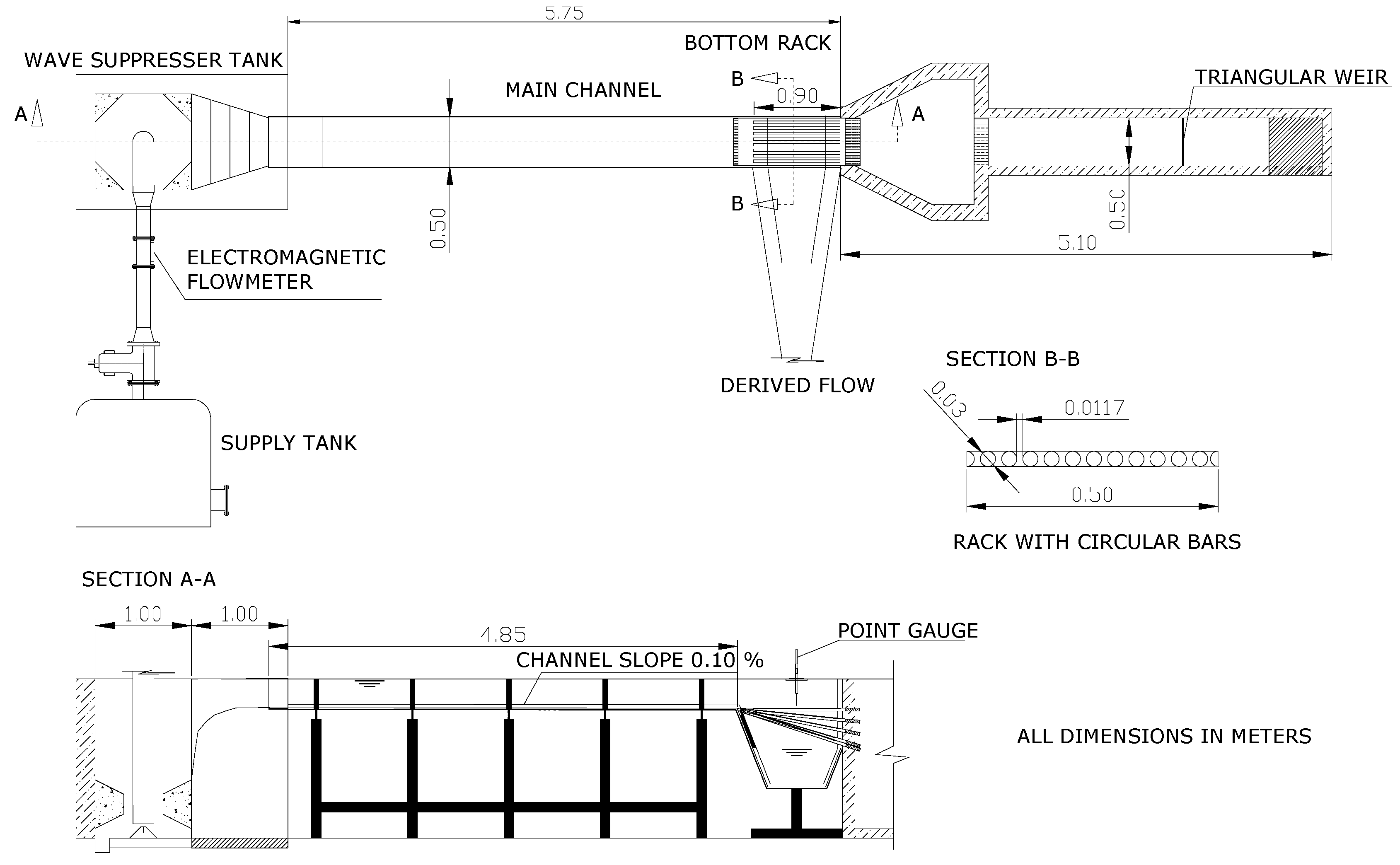
The physical device consists in an intake system based on Noseda’s [12] physical model (Figure 2). It consists of a 5.00 m long and 0.50 m wide inlet channel with methacrylate walls that allows for the inspection of the flow. At the end of the channel there is a bottom rack intake system with different slopes (from horizontal to 33%). The racks were built with aluminum bars with circular profiles (∅30 mm).
The rack length was 0.90 m with the bars horizontally oriented with the flow direction. The spacing between bars was 11.70 mm. With those considerations, the void ratio analyzed was m = 0.28. This void ratio matches with the previously analyzed racks made of T-profile bars (Carrillo et al. [22]).
Water depths were measured with a point gauge (accuracy ± 0.5 mm). The superficial flow profile was measured in the vertical planes over a bar and over the spacing between bars, from −0.50 m upstream of the beginning of the rack to the X cross-section where the flow depth was less than 2 mm.
Five longitudinal rack slopes (from 0 to 33%) and six different specific flows (from 53.8 to 198.8 l/s/m) were tested. In each experiment, the entrain specific flow q1 flow was measured with an electromagnetic flowmeter Endress Häuser Promag 53W of 125 mm with an accuracy of 0.5%, the specific discharge flow, q2, was obtained with a calibrated v-notch, while the specific discharge flow collected in the intake system, qd, was obtained as the difference between the inlet and discharged flows. Further details of the model may be obtained in García [10] and in Castillo et al. [3].
The approaching flow is subcritical in all the cases at the beginning of the inlet channel. The flow reaches supercritical conditions at the beginning of the rack. Brunella et al. [2] proposed an expression to calculate the critical Reynolds number in the bottom intake systems. According to those authors, there are no scaling effects when this value is bigger than 250,000. In the tests carried out, the critical Reynolds number at the beginning of the rack was between 186,000 and 589,000, while the Froude number at the beginning of the rack was between 1.43 and 1.81. Thus, scale effects are not expected in our tests for flows greater than 75 l/s/m.
3. Numerical Modelling
The computational fluid dynamics (CFD) programs solve the fluid mechanic problems, providing lots of data, increased profitability, flexibility, and speed than that obtained with experimental procedures. They allow us to simulate the interaction among different fluids as a two-phase air-water flow. However, the mathematical models still present accuracy issues when modelling some hydraulic phenomena (Chanson & Gualtieri [39]; Bombardelli [18]). Hence, it is necessary to validate numerical results with data obtained in prototypes or physical models (Blocken & Gualtieri [19]).
Laboratory measurements were considered to model and validate CFD simulations in order to analyze the behavior of the bottom racks. The finite-volume scheme program ANSYS CFX (version 18.0) was used. This program was previously used for solving T-shape bars in intake systems, with accurate results (Carrillo et al. [22]).
For the turbulent flow, CFD codes solve the differential Reynolds-averaged Navier–Stokes (RANS) equations of the phenomenon in each control volume of the fluid domain, retaining the reference quantity (mass, momentum, energy) in the three directions. The equations for conservation of mass and momentum may be written as:
where i and j are indices, xi represents the coordinates directions (i = 1 to 3 for x, y, z directions, respectively), ρ the flow density, t the time, U the velocity vector, p the pressure, presents the turbulent velocity in each direction (i = 1 to 3 for x, y, z directions, respectively), μ is the molecular viscosity, is the mean strain-rate tensor and is the Reynolds stress.
Although the RANS equations may be applied to variable-density flows, in this particular case Navier–Stokes equations were considered in their incompressible form.
3.1. Details of the Numerical Model
ANSYS CFX uses an element-based finite volume method. A mesh is used to construct finite volumes, which are used to conserve relevant quantities. All solution variables and fluid properties are stored at the nodes (mesh vertices). A control volume is constructed around each mesh node.
The program uses second order accurate approximations as much as possible. For the advection and the transient schemes, the high resolution option and the second order backward Euler were selected, respectively. Further details may be obtained in ANSYS CFX Manual [40].
Transient simulations were considered. Hence, Unsteady Reynolds-Averaged Navier–Stokes (URANS) turbulence models were used. In judging the convergence of a solution in a finite-volume scheme, ANSYS CFX monitors the residuals for each equation at the end of each time step. Residuals are a measure of the local imbalance of each conservative control volume equation. The solution is said to have converged if the scaled residuals are smaller than pre-set values. In this work, the Root Mean Square residual values were set to 10−4 for all the variables. A fix time step of 0.05 s was considered. Around 7–8 iterations were required to reach the convergence criteria in each time step. The transient statistics were obtained once the steady state was reached.
3.2. Free Surface Modelling
A challenge in modelling two-phase flows is to discern the required level of complexity to represent different aspects of the flow (Jha & Bombardelli [41]; Bombardelli [18]).
The Eulerian-Eulerian multiphase flow homogeneous model was selected to solve the air-water two-phase flow. This a limiting case of Eulerian-Eulerian multiphase flow where all fluids share the same velocity fields, as well as other relevant fields such as pressure and turbulence. Both phases were considered continuous fluids. The sum of the volume fraction of all phases (rα) is the unit in each control volume. It may be assumed that the free surface is on the 0.5 air volume fraction.
As transported quantities are shared in the homogeneous model, ANSYS CFX uses bulk transport equations rather than individual phasic transport equations. The bulk transport equations may be derived by summing the individual phasic transport equations over all phases to give a single equation for f:
were:
being Γ the diffusion coefficient, S the source, and NP the number of phases.
Volume fractions are expected to be close to zero or unity except near the interface. To solve the interface, the free surface model was selected. This model uses a compressive discretization scheme to keep the interface sharp, reducing the smearing at the interface (see ANSYS CFX Manual [40]). The coupled volume fraction algorithm was selected. Hence, velocity, pressure, and volume factions are implicitly coupled. The surface tension model considers the surface tension force as a volume force concentrated at the interface. A surface tension coefficient of 0.072 N/m was specified. No wall adhesion was considered.
3.3. Boundary Conditions
Although the classical approach in bottom racks is two-dimensional, the phenomenon is in fact three-dimensional. Hence, three-dimensional models were considered in this study.
An Acoustic Doppler Velocimeter was used to measure the mean and turbulent velocity at the inlet condition (located 0.50 m upstream of the front edge of the rack). The average turbulent intensity was around 3%. The model boundary conditions corresponded to the flow, the turbulence at the inlet condition, the upstream and downstream water levels, and their hydrostatic pressures distributions. The water level height was modified according to the values obtained in the laboratory device. In the upper outlet and in the outlet to the water collected channel, the flow is supercritical. Opening boundary conditions were considered. In the upper boundary, opening condition with zero gradient was considered.
Different authors have obtaining in their results that all the bars have similar behavior. For instance, García [10] shows the comparison of the flow profiles over all the racks and the spacing between bars for different inlet flows and rack slopes. Differences were scarce between bars. Following these ideas, it was considered that the longitudinal bars have the same behavior in the intake system. Hence, the fluid domain considers three bars and two spacings between bars. Symmetry conditions were used in the central plane of the extreme bars (Figure 3).
No slip wall conditions and smooth walls were considered in the solid limits. The atmosphere condition was simulated as an opening condition with a relative pressure of 0 Pa, a water volume fraction of 0, and an air volume fraction of 1.
3.4. Mesh Size Independence
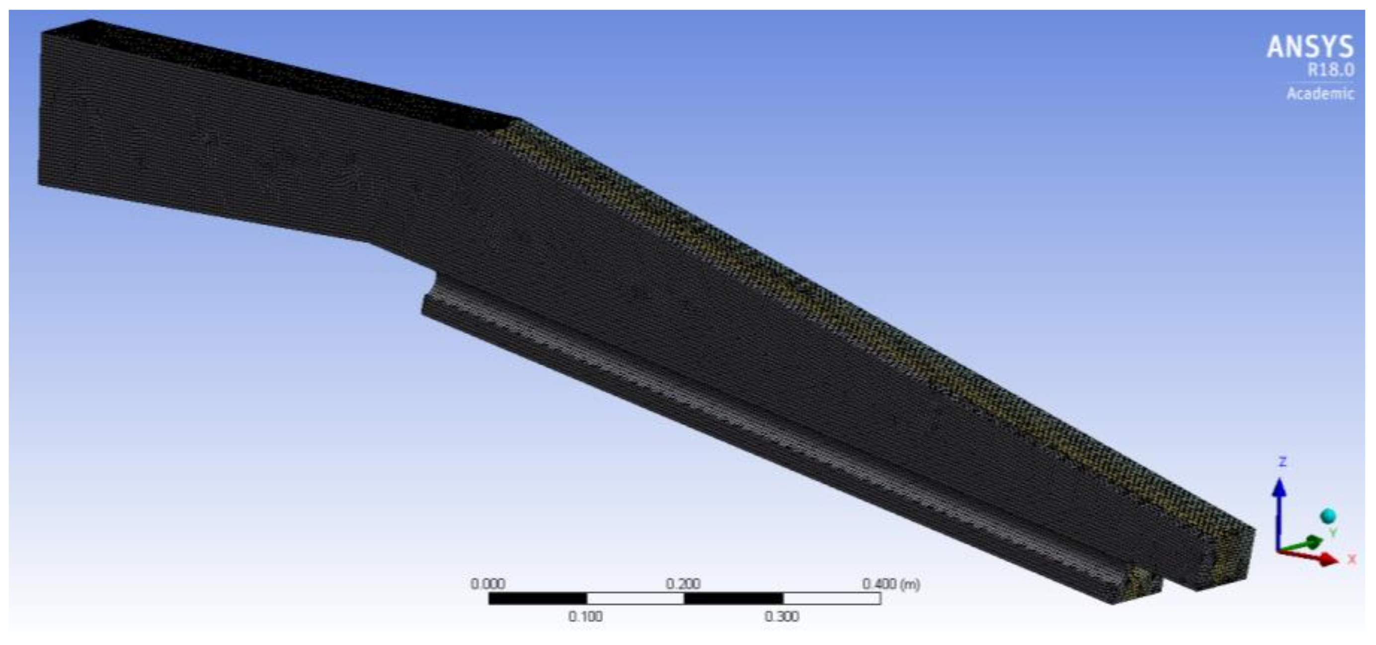
The code is based on an element-oriented, finite-volume method. It can solve different types of elements, including tetrahedral (4 nodes) and hexahedral (8 nodes) elements. Solution variables are stored at the nodes. The ratio of elements per node is approximately 5:1 for a tetrahedral mesh and 1:1 for hexahedral mesh. A tetrahedral mesh has about two times the required memory of a hexahedral mesh with the same number of nodes. More details are given in the ANSYS CFX Manual [40]. In this research, hexahedral mesh elements were considered (Figure 4).
To test the accuracy of the numerical simulations data, the flow profiles along the rack were compared by using different mesh sizes and thus obtaining mesh sizes sufficiently insensitive to the results. Table 2 shows the number of elements and the mean time required to solve the simulations using an 8-core Intel(R) Xeon(R) CPU at 2.40GHz.
For testing the mesh convergence, the Grid Convergence Index (GCI) (Roache [42]) was computed using the mesh sizes shown in Table 2. With three mesh sizes, it may be considered an optimistic safety factor, Fs = 1.25 (ASCE [43]). The analysis was based on the water depths obtained at the beginning of the spacing between bars (cross section X = 0.00 m), giving GCI values of less than 1.5% for the test carried out. The GCI is not a direct measurement of the mesh accuracy, however, it does ensure with a level of confidence that the solution is approaching to the mesh convergence solution. The comparison with the laboratory measurements also shows good agreement. Table 3 shows the GCI calculations for an inlet specific flow of 114.6 l/s/m and a rack slope of 20%.
Figure 5 compares the flow profiles over the center of the bars simulated with the three mesh sizes and the values measured in the laboratory. No differences were observed between the numerical flow profiles over the bars. The water profiles obtained with the CFD were quite similar to the laboratory measurements. The water depths obtained with the 0.006 m mesh size tend to be slightly bigger than the measurements and the other mesh sizes. However, there are no remarkable differences between the results obtained with the 0.005 and 0.004 m mesh sizes.
As there are no outstanding differences between the results obtained with the intermediate and the smaller mesh size, the 0.004 m mesh size was used to analyze the different specific flows and rack slopes. This mesh size was previously used in the numerical modelling of T-shape bars (Carrillo et al. [22]). Figure 6 shows the water depth discretization along the rack of the free surface model with the 0.004 m mesh size.
3.5. Turbulence Models
To solve the Navier–Stoke equations in reasonable time, turbulence models have been used. RANS-based turbulence models are widely used as a compromise between accuracy and computational effort. The Eddy-viscosity turbulence models consider that such turbulence consists of small eddies that are continuously forming and dissipating, and in which the Reynolds stresses are assumed to be proportional to mean velocity gradients.
The Reynolds stresses obtained in the closure problem may be related to the mean velocity gradients and eddy viscosity by the gradient diffusion hypothesis:
with µt being the eddy viscosity or turbulent viscosity, the turbulent kinetic energy and δ the Kronecker delta function.
Three of the most usual two-equation RANS-based turbulence models have been tested to solve the flow in the surrounding of the bottom racks: the standard k-ε model (Launder & Sharma [44]), the Re-Normalization Group (RNG) k-ε model (Yakhot & Smith [45]), and the k-ω based Shear-Stress Transport (SST) model (Menter [46]). For the k-ε models, scalable wall functions were considered. For the SST model, automatic wall functions were considered. The y+ value was smaller than 200 in all the simulations. More details are given in the ANSYS CFX Manual [40].
3.6. Turbulence Model Comparison
Due to the different behavior of the turbulence models in flow separation, the influence of the turbulence model has also been tested with three of the most widely used turbulence models: the standard k-ε, the Re-Normalization Group (RNG) k-ε model, and the Shear-Stress Transport (SST) model.
Figure 7 compares the values of the flow profiles over the center of the circular bars. For the cases considered, the solution seems to be dominated by the gravity. There are no outstanding differences between the three turbulence models and the laboratory measurements. Results are in agreements with the conclusions obtained in the turbulence model comparison of T-shape bars (Carrillo et al. [22]).
4. Results and Discussion
Once the results with different mesh sizes and the turbulence model had been validated, simulations were carried out with five specific flows and different slopes.
4.1. Flow Profile over ther Rack
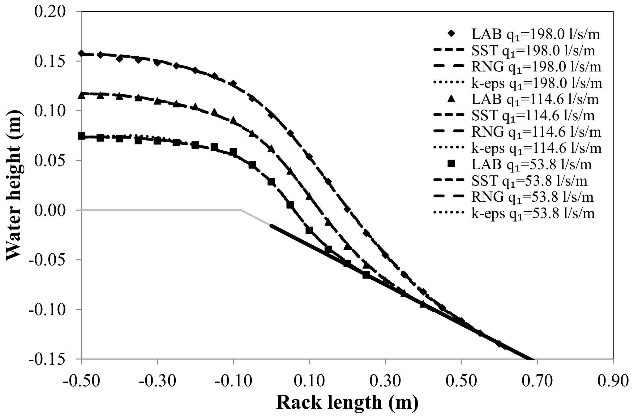
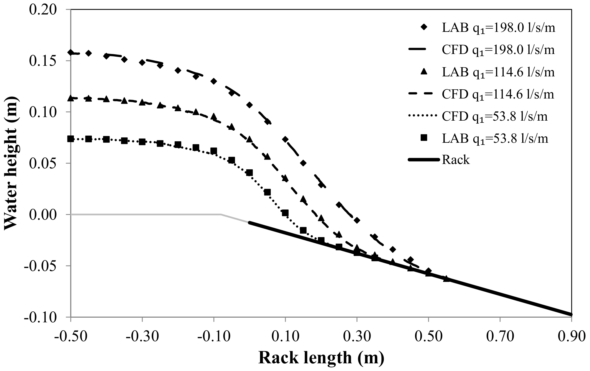
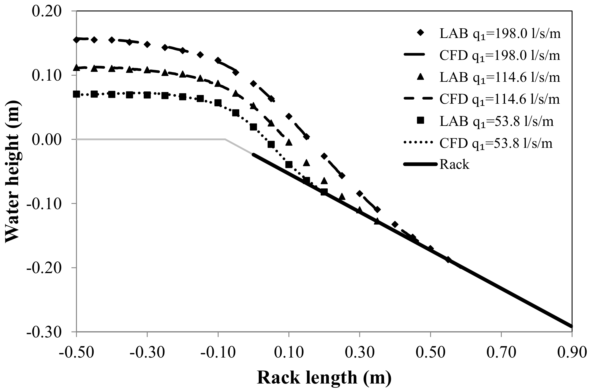
To determine the accuracy of the numerical simulations in comparison with the laboratory measurements, the longitudinal flow profiles were compared. Figure 8 and Figure 9 show the longitudinal flow profiles over the center of the circular bars for three specific flows (53.8, 114.6 and 198.0 l/s/m). In both cases, the values show a good agreement.
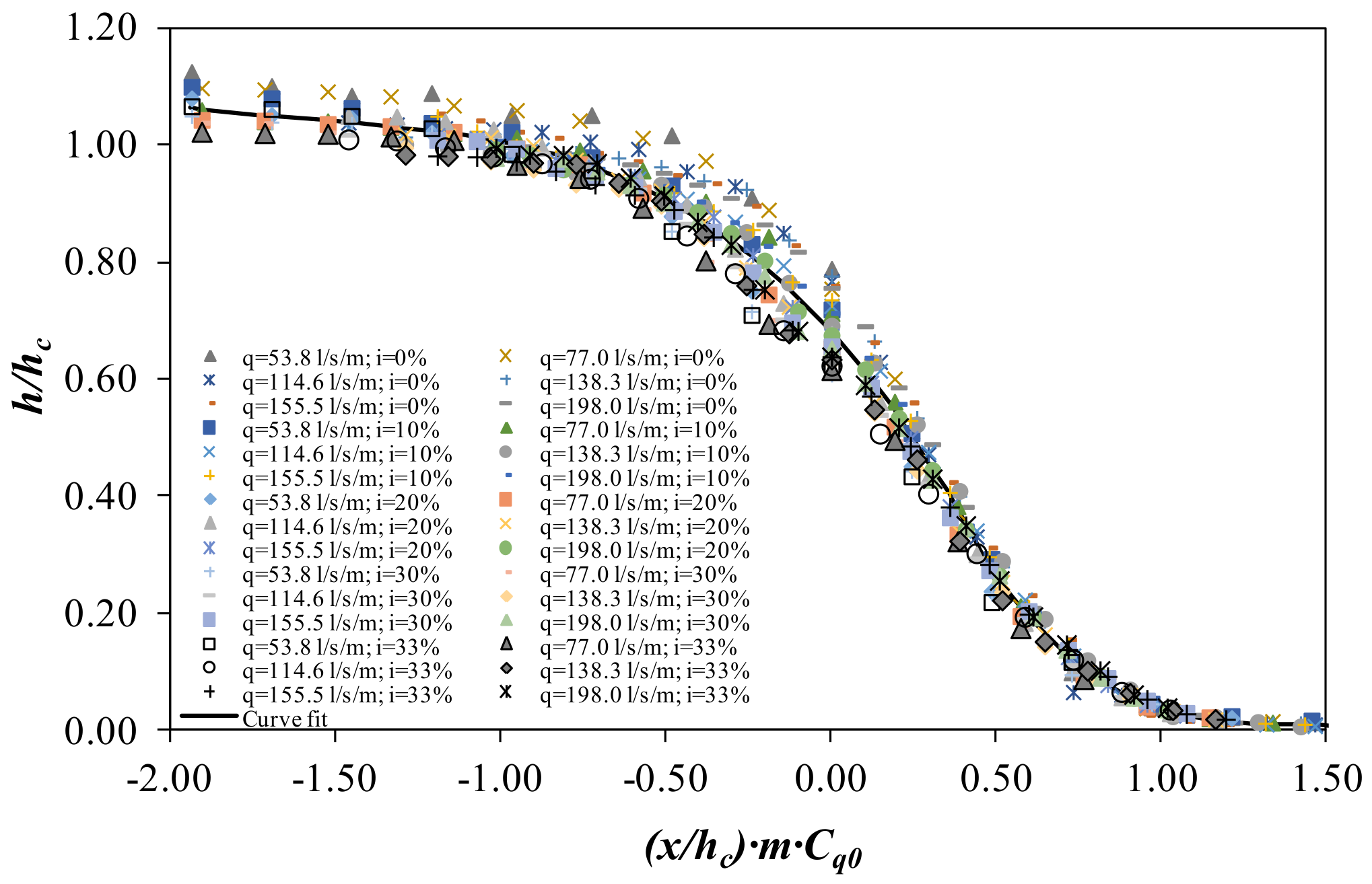
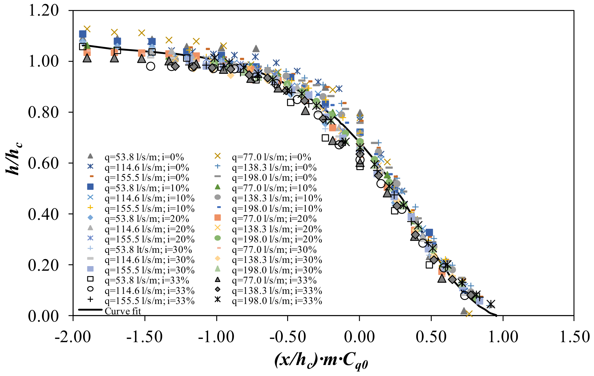
Following Brunella et al. [2], flow profiles may be compared if the values are shown in a dimensionless way, considering the critical depth hc, the void ratio m, and the discharge coefficient measured in static conditions Cq0 (Castillo et al. [24,49]). Considering the 30 configurations carried out, Figure 10 and Figure 11 show the non-dimensional flow profiles over the bar and over the spacing between bars.
The trend is the same in both flow profiles for x/hc · m · Cq0 < 0.50. For values greater than 0.50, the behavior over the bars and over the spacing between bars seems to follow different fit curves. Figure 10 and Figure 11 also show polynomial curve fits with r2 > 0.95:
The coefficients of the 4th order fits are shown in Table 4.
4.2. Wetted Rack Length
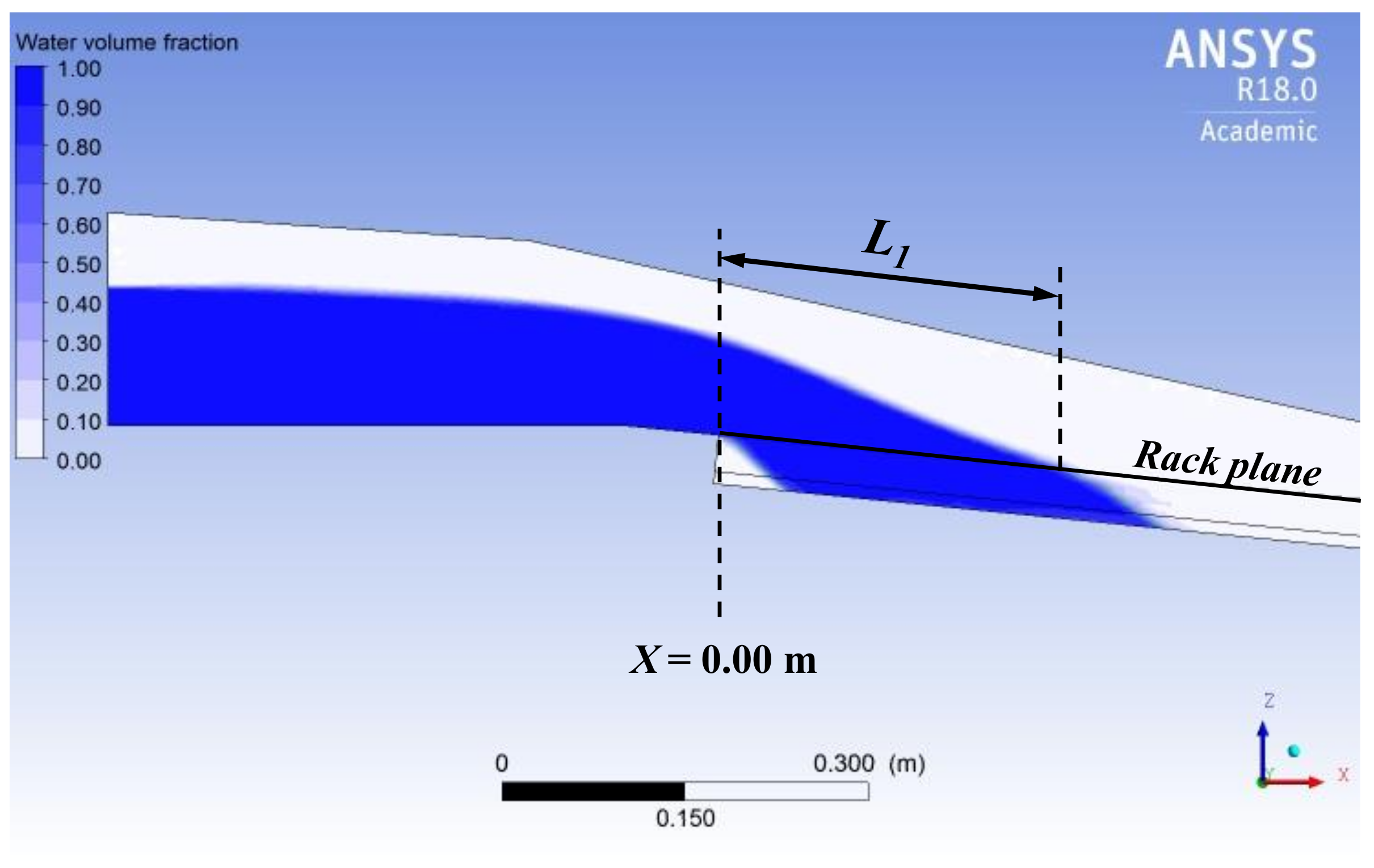
Designers need to be able to estimate the minimum length of the rack necessary to derive a determinate flow (García et al. [50]). Drobir et al. [8] defined L1 as the distance from the beginning of the rack to the section where the nappe enters directly through the racks (measured between the bars) (Figure 12).
The L1 values have been obtained in the laboratory device and in the numerical simulations considering different specific flows and slopes. Table 5 and Table 6 show the comparison of measured and simulated length values. Despite the good behavior shown in the flow profiles (with a relative error of around 1%), the spacing between bars is a challenge region for the free surface modelling. Maximum differences were around 4% of the laboratory value for all the cases considered.
4.3. Discharge Coefficient
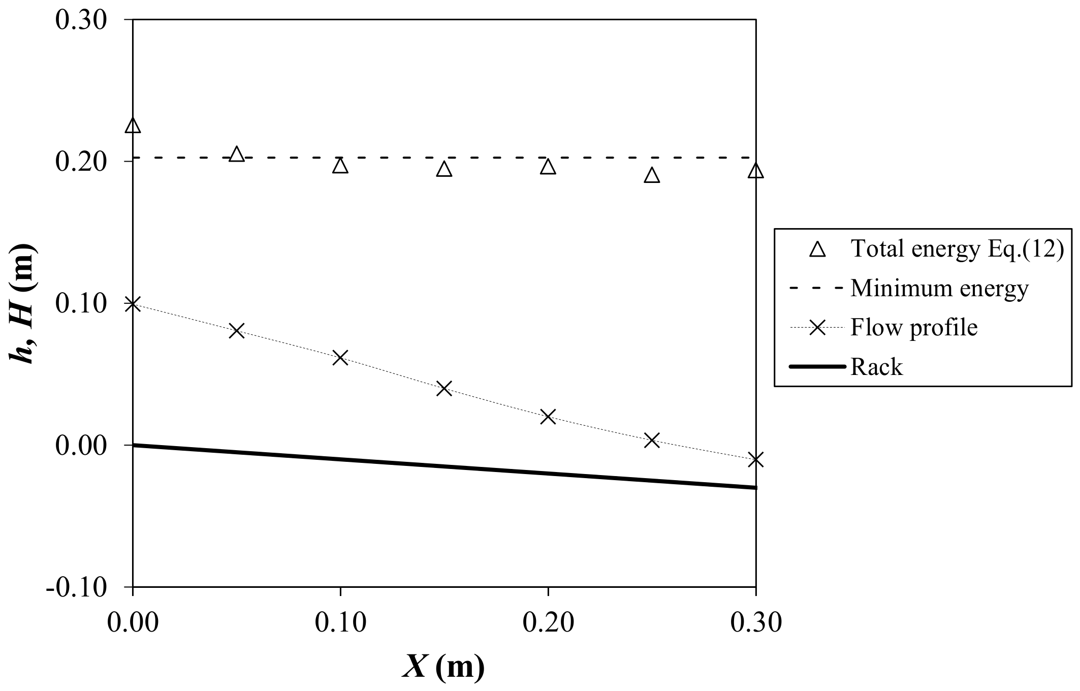
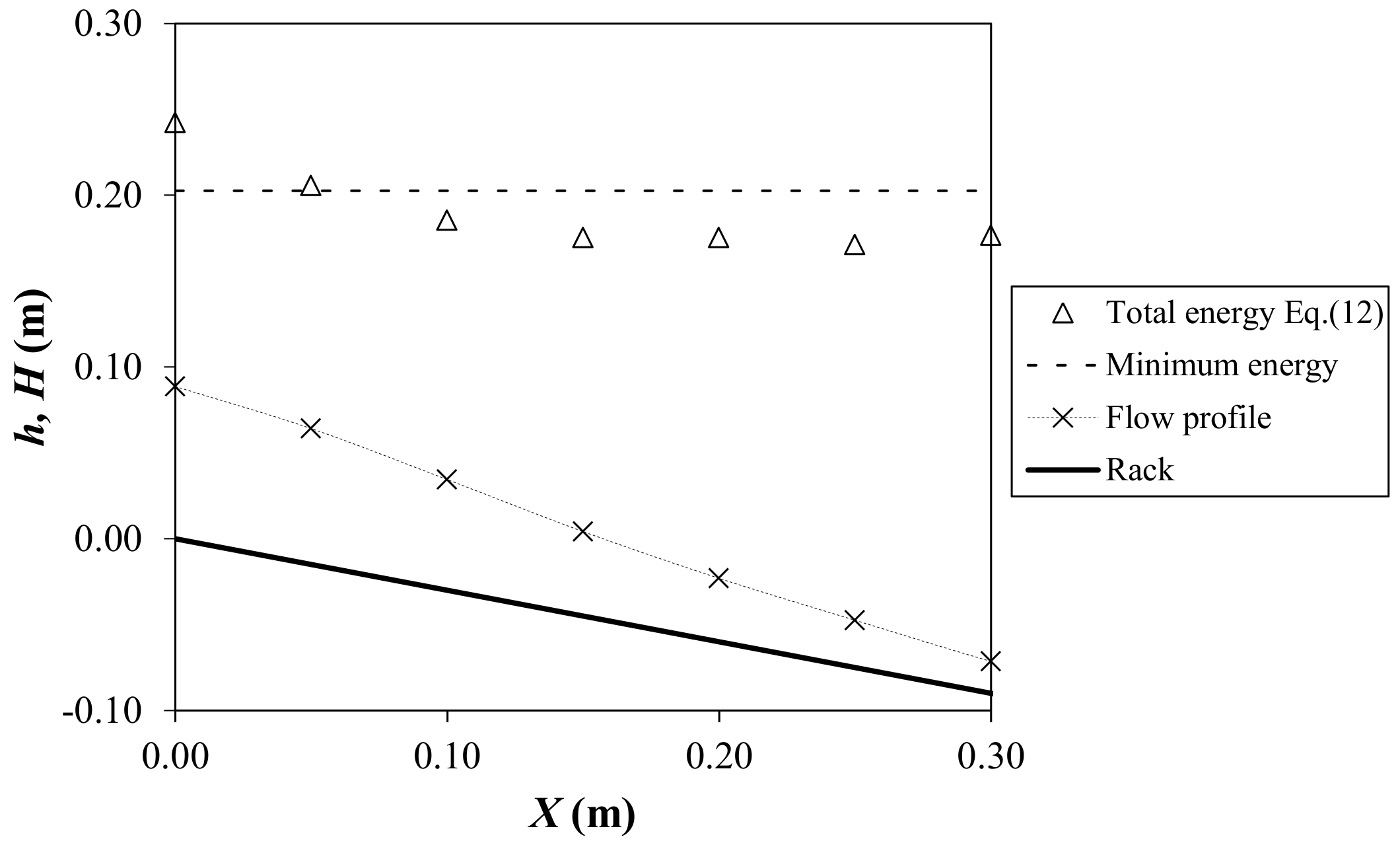
To solve the flow over the rack, there are two classical approaches, considering the energy level horizontal or parallel to the rack plane. The total energy H may be calculated in each cross-section to analyze which approach is more accurate,
where z is the vertical distance from the datum.
Figure 13 and Figure 14 show the total energy along the rack calculated for two cases, together with the measured water depth and the minimum energy at the beginning of the rack. With those results, the hypothesis of minimum energy level at the beginning of the rack may be considered a good approximation of the phenomenon.
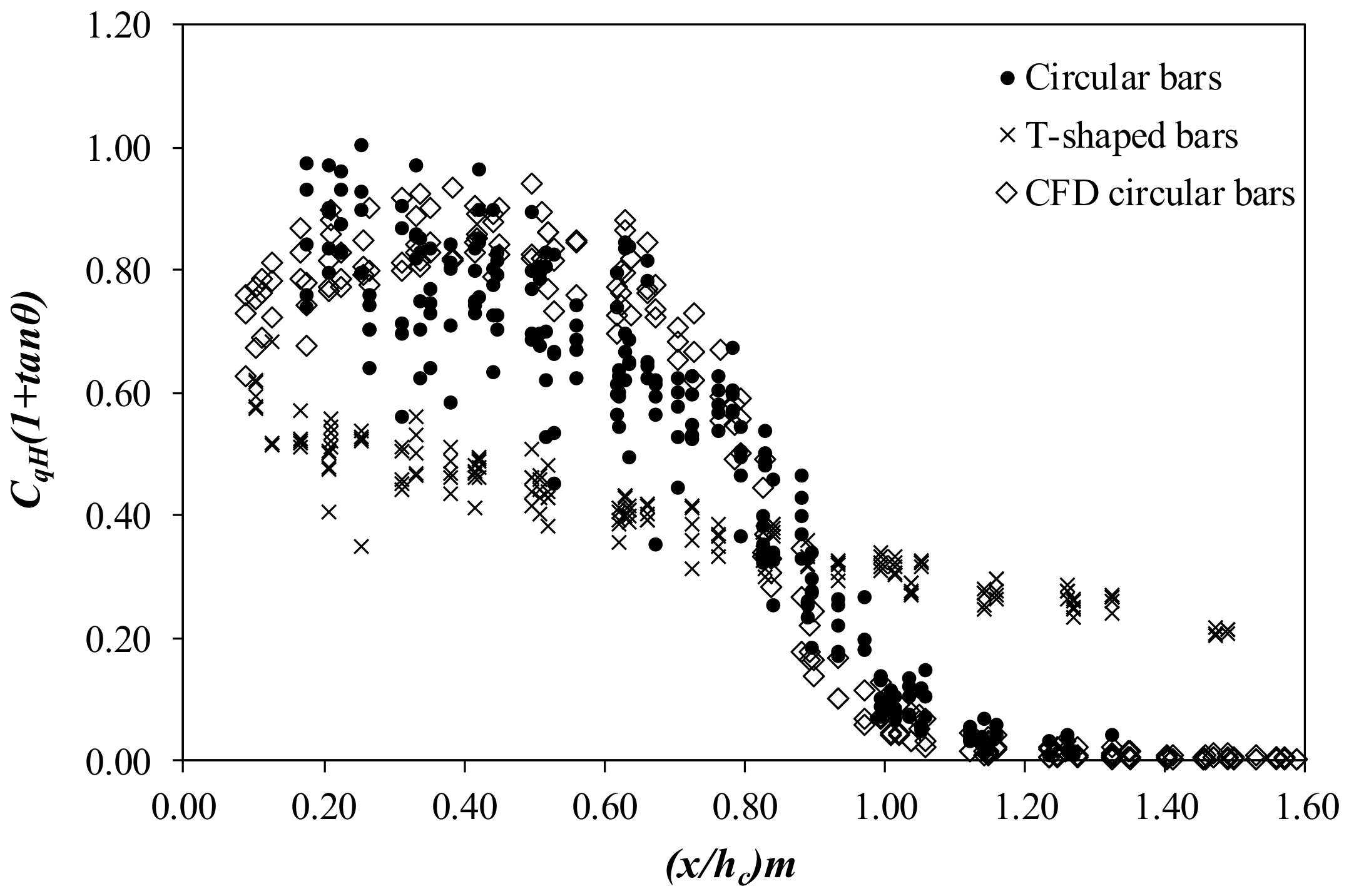
The discharge coefficient changes along the rack. Considering the horizontal energy head hypothesis and H0 = Hmin for the incoming flow, the discharge coefficient CqH along the rack has been calculated from Equation (3) using the measurements of the rejected flow at each cross-section.
Figure 15 shows the CqH variation in a dimensionless way for several flows and rack slopes. Results are similar than those obtained from CFD simulations. Values obtained with T-shaped bars have also been considered for the same void ratio (Castillo et al. [24]). There are remarkable differences among the behavior of the racks made with circular and T-shape bars. Racks with circular bars have higher values of discharge coefficients. That drives to a smaller wetted rack length to derive the same flow. However, these discharge coefficients correspond to clear water tests.
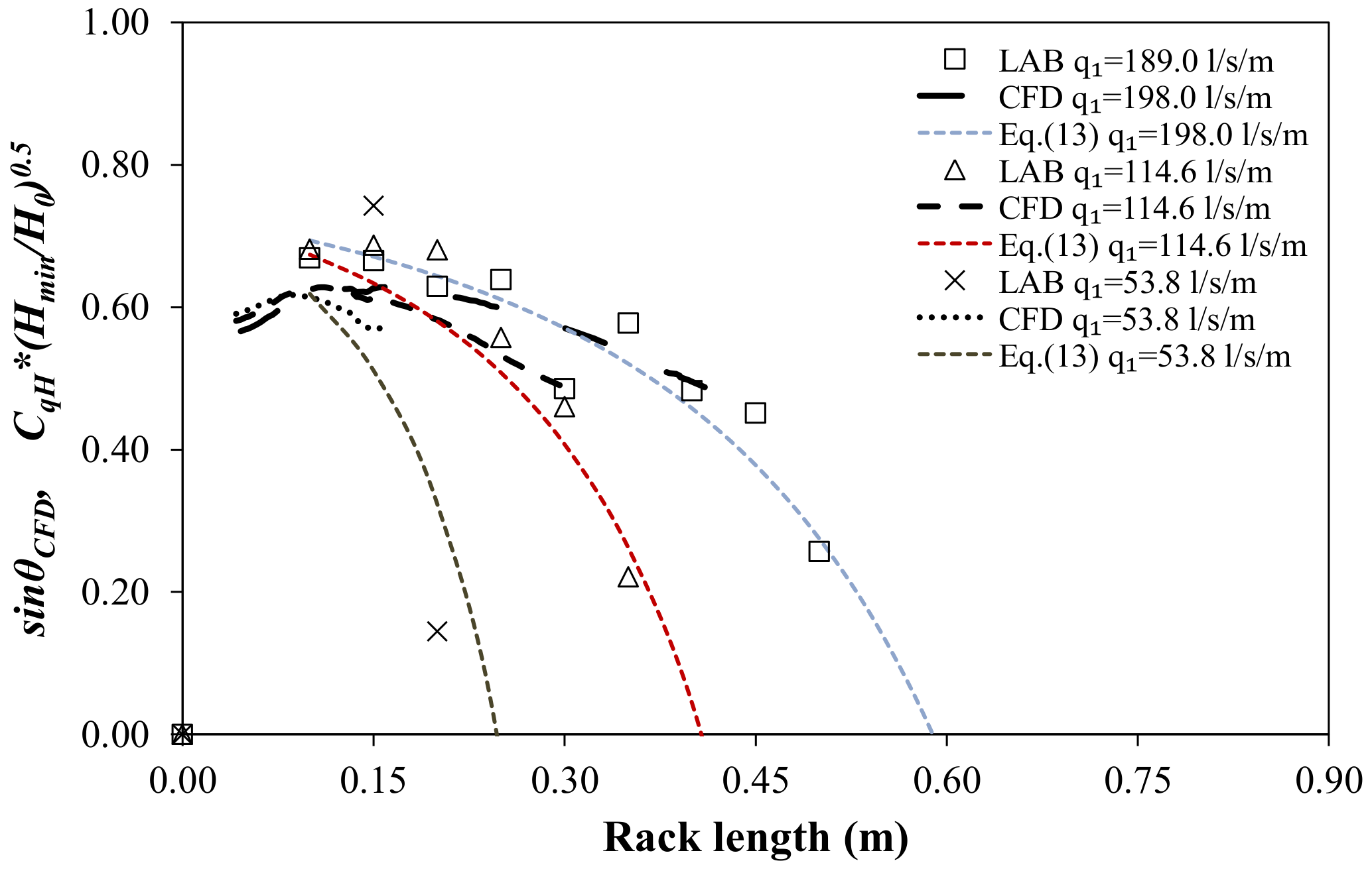
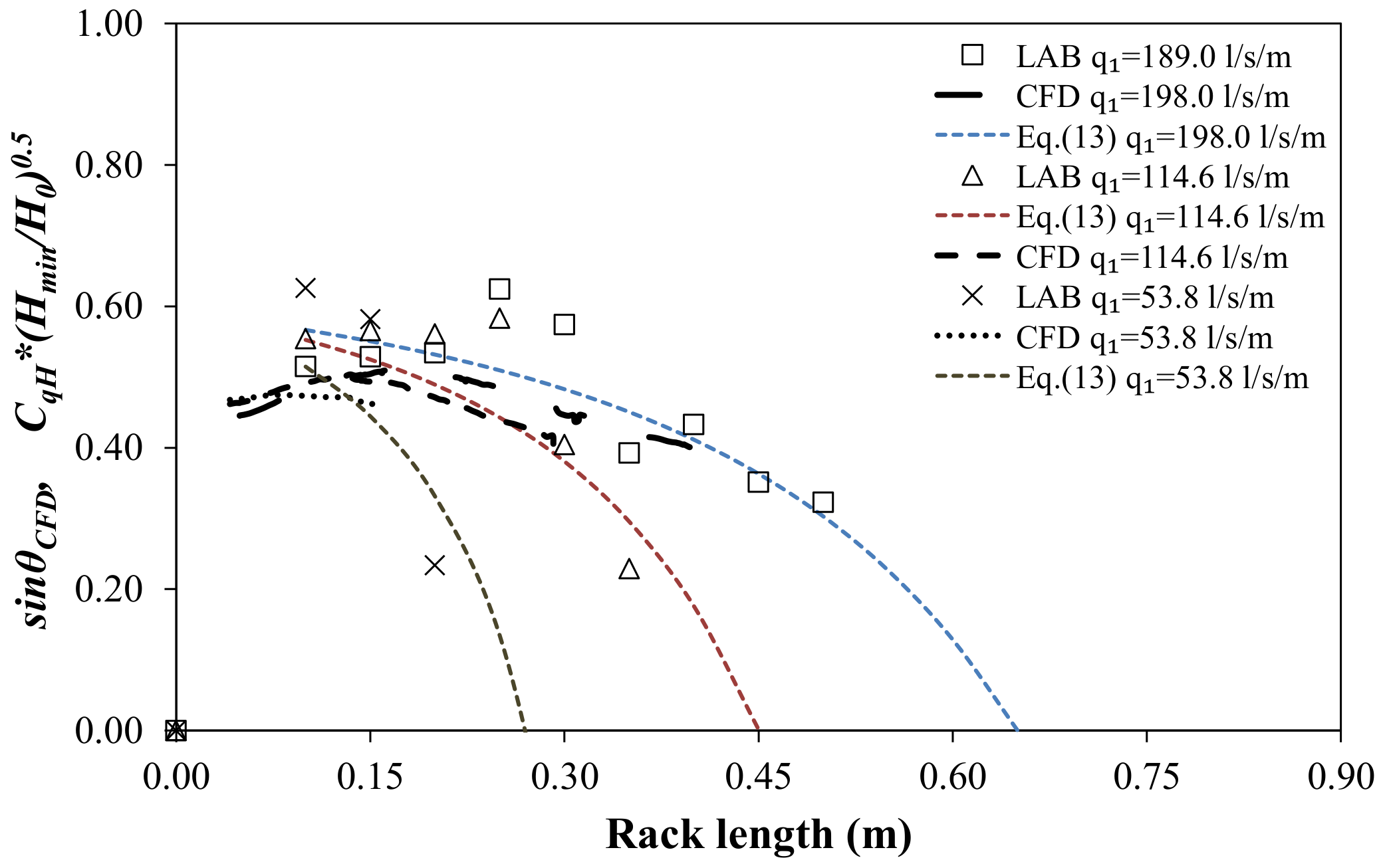
Following Righetti & Lanzoni [9], the discharge coefficient of the collected flow may be estimated using the angle of the velocity vector of water collected with the rack plane, θ. Figure 16 and Figure 17 compare the numerical results obtained for different specific flows and rack slopes. For the laboratory data, a fit curve was obtained as a function of the void ratio and the slope of the rack for the circular bars,
Equation (13) has the advantage of avoiding the requirement of the water depth along the rack to calculate the derived flow. The adjustment has been considered H0 = Hmin for the incoming flow, and horizontal energy level along the rack. The accuracy of Equation (13) will be discussed in the following section.
Table 7 shows the differences between the energy head measurements at the beginning of the rack H0, and the minimum energy Hmin. To obtain the empirical discharge coefficient related to the real energy head, Equation (13) has been multiplied by the square root of the ratio Hmin/H0.
Although there are different bars types and flow conditions from Righetti & Lanzoni [9], similar results are obtained in terms of verifying CqH ≈ sinα. While the different flows obtain similar maximum CqH values, the rack slope seems to influence the maximum. In this way, smaller maximum CqH values are obtained with bigger rack slopes. After the maximum, the discharge coefficient tends to reduce with the decreasing of the water depth over the rack. Differences with the empirical formula proposed in Equation (13) are related with the consideration that the energy remains constant along the rack.
4.4. Water Collected
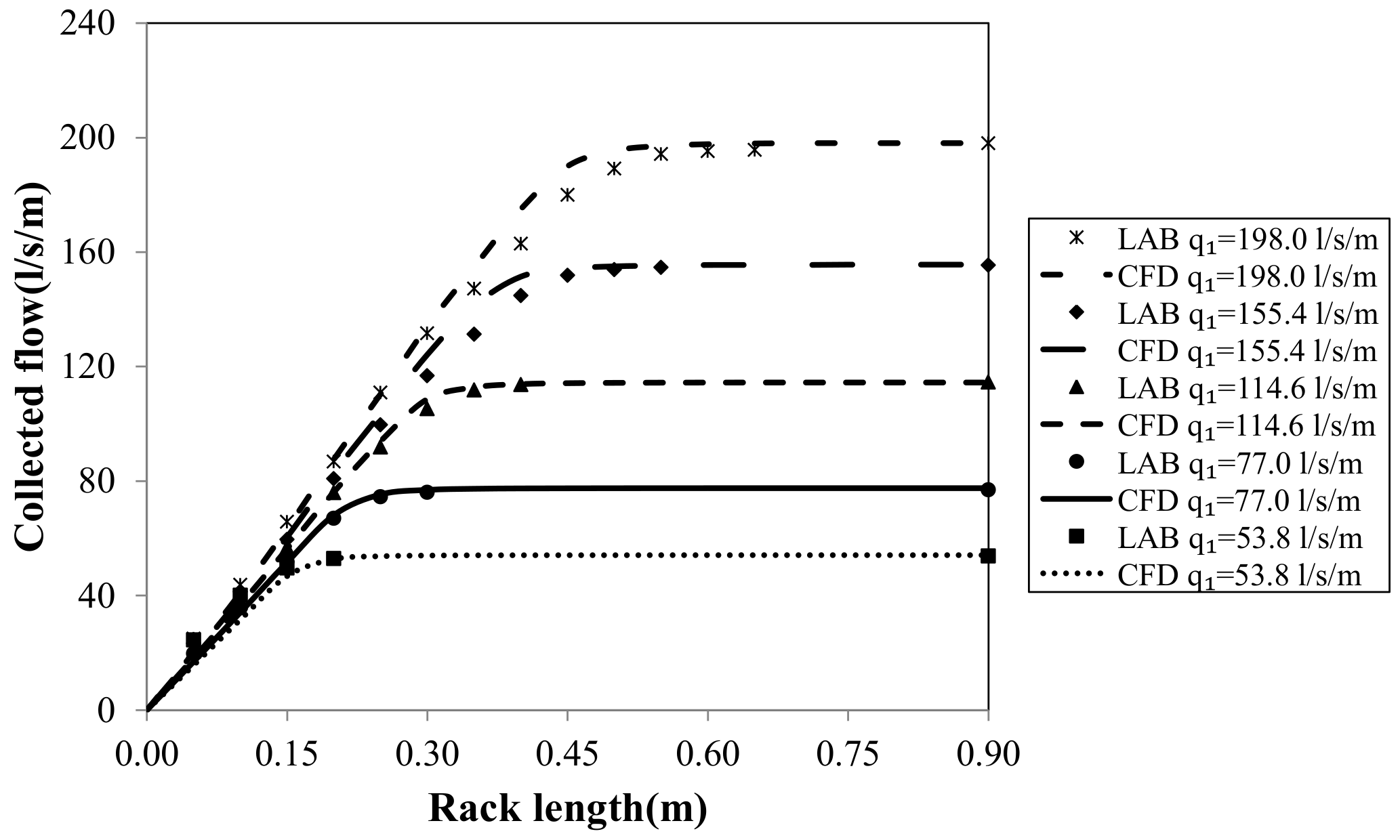
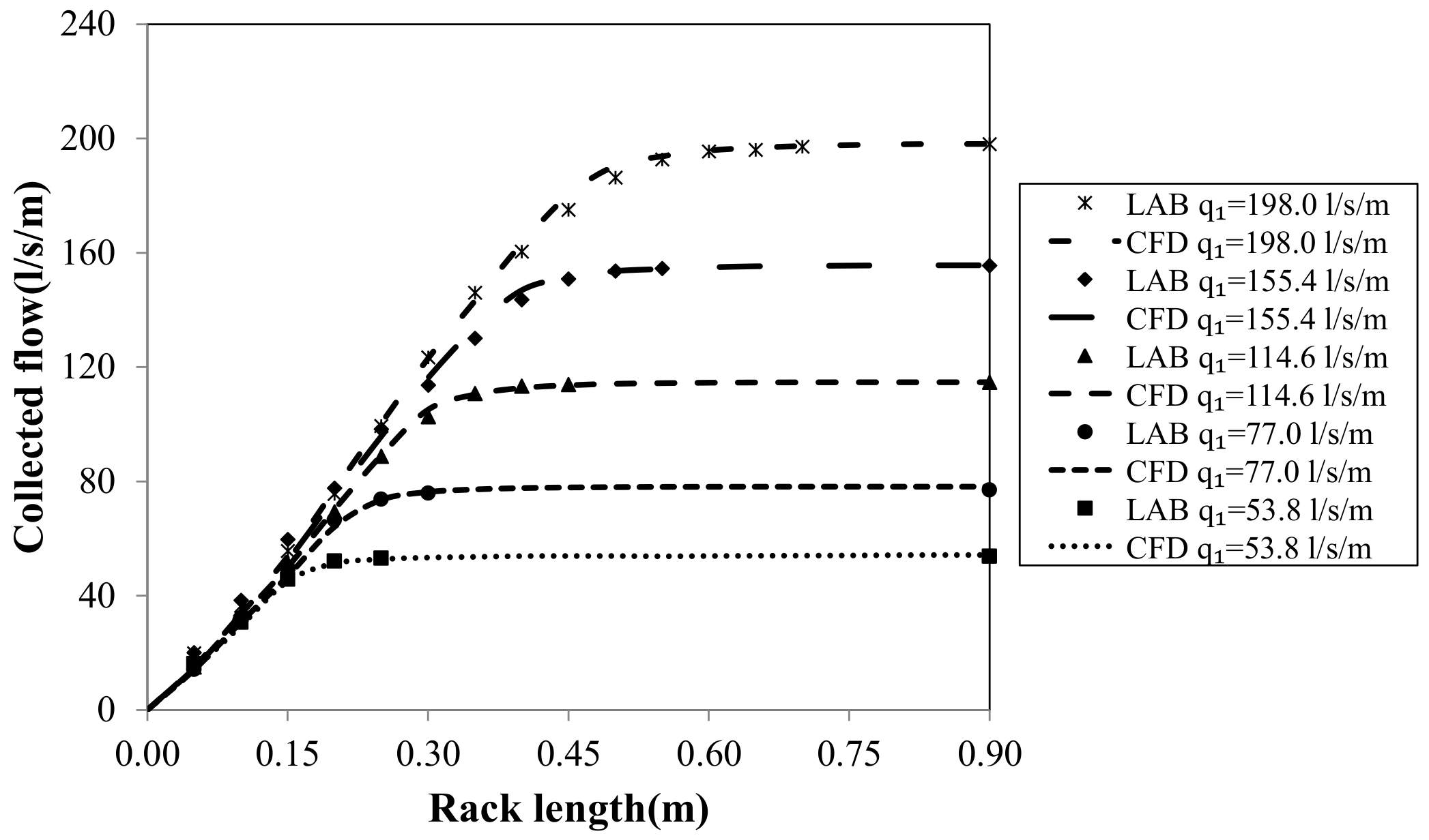
Figure 18 and Figure 19 compare the laboratory and numerical water collected along the rack length for five specific flows and two different rack slopes. In both cases, the flow entrain-flow collected ratio is quite similar. With the smaller rack slope and the highest specific flow, the differences tend to increase until reaching maximum differences smaller than 5%. This may be related with the observed differences in the streamlines in the zone of maximum curvature, the discrepancies in the wetted rack length (maximum differences around 4%), and the random errors of the physical device (including the flowmeter, the point gauge, and the triangular weir measurements).
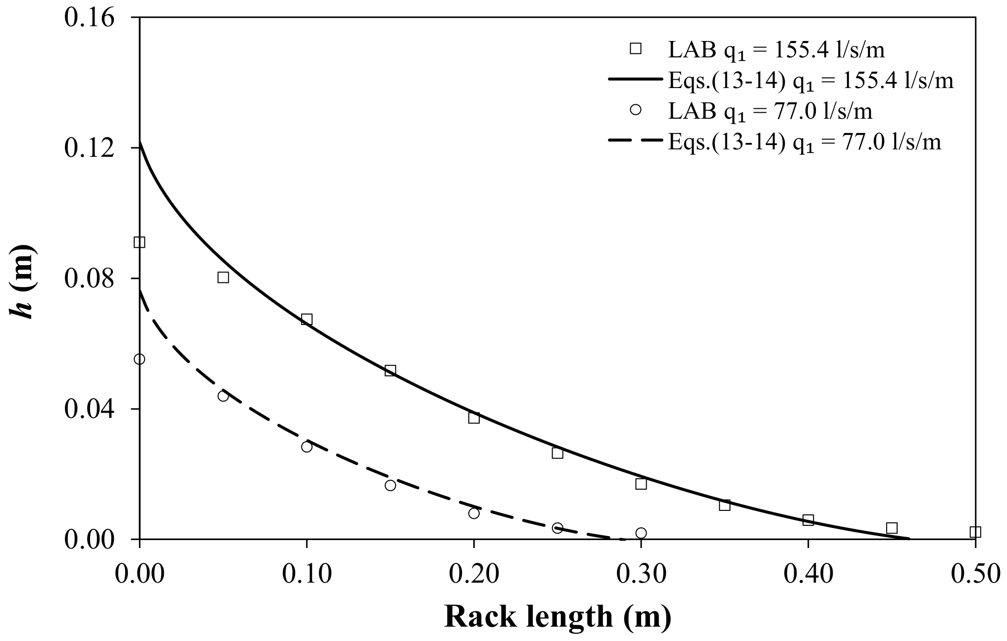
Figure 20 shows the comparison between the measured values of the flow profile and the cumulative derived flow, with those numerically solved from Equations (3) and (13) with a fourth order Runge–Kutta method, obtaining
In general, the flow profiles show a good agreement between measured and numerically simulated values using the discharge coefficient proposed in Equation (13). Figure 21 shows the comparison between experimental and solved cumulative derived flow. Differences are smaller than 3%.
5. Conclusions
Bottom racks are traditionally used in stepped streams to obtain water, minimizing the sediment collected and the maintenance of the intake system.
The required rack length to collect a desirable flow is one of the key parameters in this type of system. However, the length may vary up to twofold as a function of the author selected.
To limit the uncertainty, numerical simulations appear to be a helpful tool to design the right intake system. However, nowadays it is required to compare numerical results with experimental and field data. In this work, the accuracy of ANSYS CFX to solve bottom racks has been tested in the clear water case. Simulations have been compared with laboratory data at the same scale. After the validation of the meshing, it may be concluded that elements of 0.004 m drive to results independently of the mesh size. Smaller mesh sizes would require more computational effort without outstanding differences in the main results.
Due to the different behavior of the turbulence models with flow separation, three of the most widely used turbulence models have been considered. With the tests carried out, the results obtained are almost the same, with no significant differences among them.
Once the validation process has been done, different comparisons have been considered. Regarding the flow profiles over the rack, the numerical results are in agreement with the laboratory data for all the cases analyzed. In the same way, the maximum wetted rack length over the spacing diverges around 3% from the laboratory measurements. The results obtained for the water collected along the rack are also quite similar, with maximum differences of less than 5%.
The classical approaches consider the rack flow to be 2D. For design, this simplification seems to be reasonable. In this work, the different formulations have been updated for circular bars.
Considering the laboratory data, fit curves have been obtained to estimate the flow profile over the bars and over the spacing between bars. The shape of the flow profile in both longitudinal planes is the same in the first part of the rack. The adjustments in a non-dimensional way show values of r2 > 95%.
Regarding the discharge coefficient, circular bars show bigger maximum values than T-shape bars with the same void ratio. That drives to smaller requirements of rack length to collect the same flow.
Expressions have been developed to calculate the collected flow and the discharge coefficient along the rack. Good agreement has been obtained with laboratory measurements considering different inlet flows and rack slopes.
Finally, the sinus of the angle of the velocity vector of water collected with the rack plane has been considered as a discharge coefficient along the rack. The results are in agreement with previous studies.
The sediment transport increases the flow resistance. An increment in the required wetted rack length is expected to collect the same amount of water than with clear water. In this way, experiments with sediments are required to know the racks behavior in those conditions.
Author Contributions
J.M.C. carried out the numerical simulations, the data analysis, and participated in the writing. J.T.G. carried out the laboratory measurements, the data treatment, and participated in the writing. L.G.C. carried out the analysis and application of the methodology, analyzed the results, and participated in the writing. All three authors reviewed and contributed to the final manuscript.
Acknowledgments
The authors are grateful for the financial support received from the Seneca Foundation of Región de Murcia (Spain) through the project “Optimización de los sistemas de captación de fondo para zonas semiáridas y caudales con alto contenido de sedimentos. Definición de los parámetros de diseño”. Reference: 19490/PI/14.
Conflicts of Interest
The authors declare no conflict of interest.
References
- Righetti, M.; Rigon, R.; Lanzoni, S. Indagine sperimentale del deflusso attraverso una griglia di fondo a barre longitudinali. In Proceedings of the XXVII Convegno di Idraulica e Costruzioni Idrauliche, Genova, Italy, 12–15 September 2000; Volume 3, pp. 112–119. (In Italian). [Google Scholar]
- Brunella, S.; Hager, W.; Minor, H. Hydraulics of Bottom Rack Intake. J. Hydraul. Eng. 2003, 129, 2–10. [Google Scholar] [CrossRef]
- Castillo, L.G.; García, J.T.; Carrillo, J.M. Experimental and Numerical Study of Bottom Rack Occlusion by Flow with Gravel-Sized Sediment. Application to Ephemeral Streams in Semi-Arid Regions. Water 2016, 8, 166. [Google Scholar] [CrossRef]
- Bouvard, M.; Kuntzmann, J. Étude théorique des grilles de prises d’eau du type En dessous. La Houille Blanche 1954, 5, 569–574. (In French) [Google Scholar] [CrossRef]
- Frank, J.; Von Obering, E. Hydraulische Untersuchungen für das Tiroler Wehr. Der Bauing. 1956, 31, 96–101. (In German) [Google Scholar]
- Henderson, F.M.N. Open Channel Flow; MacMillan: New York, NY, USA, 1966. [Google Scholar]
- Vargas, V. Tomas de fondo. In Proceedings of the XVIII Congreso Latinoamericano de Hidráulica, Oaxaca, Mexico, 6–10 October 1998. (In Spanish). [Google Scholar]
- Drobir, H.; Kienberger, V.; Krouzecky, N. The wetted rack length of the Tyrolean weir. In Proceedings of the IAHR-28th Congress, Graz, Austria, 22–27 August 1999. [Google Scholar]
- Righetti, M.; Lanzoni, S. Experimental Study of the Flow Field over Bottom Intake Racks. J. Hydraul. Eng. 2008, 134, 15–22. [Google Scholar] [CrossRef]
- García, J.T. Estudio Experimental y Numérico de los Sistemas de Captación de Fondo. Ph.D. Thesis, Universidad Politécnica de Cartagena, Murcia, Spain, 2016. (In Spanish). [Google Scholar]
- Chaguinov, G.N. Prise d’eau du type tyrolien. Thèse, Moscow, 1937. (In French). [Google Scholar]
- Noseda, G. Correnti permanenti con portata progressivamente decrescente, defluenti su griglie di fondo. L’Energ. Elettr. 1956, 33, 41–51. (In Italian) [Google Scholar]
- Noseda, G. Correnti permanenti con portata progressivamente decrescente, defluenti su griglie di fondo. L’Energ. Elettr. 1956, 33, 565–588. (In Italian) [Google Scholar]
- Gherardelli, S. Sul calcolo idraulico delle griglie di fondo. L’Energ. Elettr. 1956, 1347. (In Italian) [Google Scholar]
- Motskow, M. Sur le calcul des grilles de prise d’eau. La Houille Blanche 1957, 12, 570–580. (In French) [Google Scholar]
- Dagan, G. Notes sur le calcul hydraulique des grilles par-dessous. La Houille Blanche 1963, 18, 59–65. (In French) [Google Scholar] [CrossRef]
- Krochin, S. Diseño Hidráulico, 2nd ed.; EPN: Ecuador, Quito, 1978; pp. 97–106. (In Spanish) [Google Scholar]
- Bombardelli, F.A. Computational multi-phase fluid dynamics to address flows past hydraulic structures. In Proceedings of the 4th IAHR International Symposium on Hydraulic Structures, Porto, Portugal, 9–11 February 2012. [Google Scholar]
- Blocken, B.; Gualtieri, C. Ten iterative steps for model development and evaluation applied to Computational Fluid Dynamics for Environmental Fluid Mechanics. J. Environ. Model. Softw. 2012, 33, 1–22. [Google Scholar] [CrossRef]
- Zerihun, Y.T. Numerical simulation of flow in open channels with bottom intake racks. Water Util. J. 2015, 11, 49–61. [Google Scholar]
- Hosseini, K.; Rikhtegar, S.; Karami, H.; Bina, K. Application of Numerical Modeling to Assess Geometry Effect of Racks on Performance of Bottom Intakes. Arab. J. Sci. Eng. 2015, 40, 677–687. [Google Scholar] [CrossRef]
- Carrillo, J.M.; Castillo, L.G.; García, J.T.; Sordo-Ward, A. Considerations for the design of bottom intake systems. J. Hydroinform. 2018, 20, 232–245. [Google Scholar] [CrossRef]
- Castillo, L.G.; Carrillo, J.M. Comparison of methods to estimate the scour downstream of a ski jump. Int. J. Multiph. Flow 2017, 92, 171–180. [Google Scholar] [CrossRef]
- Castillo, L.G.; García, J.T.; Carrillo, J.M. Influence of rack slope and approaching conditions in bottom intake systems. Water 2017, 9, 65. [Google Scholar] [CrossRef]
- Garot, F. De Watervang met liggend rooster. De Ingenieur in Nederlandsch Indie 1939, 6, 115–132. (In German) [Google Scholar]
- Orth, J.; Chardonnet, E.; Meynardi, G. Étude de grilles pour prises d’eau du type ‘en-dessous. La Houille Blanche 1954, 9, 343–351. (In French) [Google Scholar] [CrossRef]
- White, J.K.; Charlton, J.A.; Ramsay, C.A.W. On the design of bottom intakes for diverting stream flows. In Proceedings of the Institution of Civil Engineers, London, UK, 18–21 April 1972; Volume 51, pp. 337–345. [Google Scholar] [CrossRef]
- Ract-Madoux, M.; Bouvard, M.; Molbert, J.; Zumstein, J. Quelques réalisations récentes de prises en-dessous à haute altitude en Savoie. La Houille Blanche 1955, 10, 852–878. (In French) [Google Scholar] [CrossRef]
- Drobir, H. Entwurf von Wasserfassungen im Hochgebirge. Österreichische Wasserwirtschaft 1981, 11, 243–253. (In German) [Google Scholar]
- Bouvard, M. Mobile Barrages and Intakes on Sediment. Transporting Rivers: IAHR Monograph Series; Balkema, A.A., Ed.; Routledge: London, UK, 1992. [Google Scholar]
- Raudkivi, A.J. Hydraulic Structures Design Manual; IAHR Monograph; Taylor & Francis Group: Abingdon Oxon, UK, 1993; pp. 92–105. [Google Scholar]
- Castillo, L.G.; García, J.T.; Carrillo, J.M. Experimental measurements of flow and sediment transport through bottom racks-influence of gravels sizes on the rack. In Proceedings of the International Conference on Fluvial Hydraulics, Lausanne, Switzerland, 3–5 September 2014; pp. 2165–2172. [Google Scholar]
- Bina, K.; Saghi, H. Experimental study of discharge coefficient and trapping ratio in mesh-panel bottom rack for sediment and non-sediment flow and supercritical approaching conditions. J. Exp. Therm. Fluid Sci. 2017, 88, 171–186. [Google Scholar] [CrossRef]
- De Marchi, G. Profili longitudinali della superficie libera delle correnti permanenti lineari con portata progressivamente crescente o progressivamente decrescente entro canali di sezione constante. Ric. Sci. Ricostr. 1947, 203–208. (In Italian) [Google Scholar]
- Nakagawa, H. On Hydraulic Performance of Bottom Diversion Works; Bulletin of Disaster Prevention Research Institute, Kyoto University: Kyoto, Japan, 1969. [Google Scholar]
- Ahmad, Z.; Mittal, M.K. Hydraulic design of trench weir on Dabka River. Water Energy Int. 2003, 60, 28–37. [Google Scholar]
- Ghosh, S.; Ahmad, Z. Characteristics of flow over bottom racks. Water Energy Int. 2006, 63, 47–55. [Google Scholar]
- Kumar, S.; Ahmad, Z.; Kothyari, U.C.; Mittal, M.K. Discharge characteristics of a trench weir. Flow Meas. Instrum. 2010, 21, 80–87. [Google Scholar] [CrossRef]
- Chanson, H.; Gualtieri, C. Similitude and scale effects of air entrainment in hydraulic jumps. J. Hydraul. Res. 2008, 46, 35–44. [Google Scholar] [CrossRef]
- ANSYS Inc. ANSYS CFX. Solver Theory Guide. Release 18.0; ANSYS, Inc.: Southpointe, Canonsburg, PA, USA, 2016. [Google Scholar]
- Jha, S.K.; Bombardelli, F.A. Toward two-phase flow modeling of non-dilute sediment transport in open channels. J. Geophys. Res. Earth Surf. 2010, 115, 2003–2012. [Google Scholar] [CrossRef]
- Roache, P.J. Quantification of uncertainty in computational fluid dynamics. Annu. Rev. Fluid. Mech. 1997, 29, 123–159. [Google Scholar] [CrossRef]
- ASCE. Verification and Validation of 3D Free-Surface Flow Models. Task Committee on 3D Free-Surface Flow Model Verification and Validation; Environmental and Water Resources Institute (EWRI): Reston, VA, USA, 2009. [Google Scholar]
- Launder, B.E.; Sharma, B.I. Application of the energy dissipation model of turbulence to the calculation of flow near a spinning disc. Lett. Heat Mass Transf. 1972, 1, 131–138. [Google Scholar]
- Yakhot, V.; Smith, L.M. The renormalization group, the ɛ-expansion and derivation of turbulence models. J. Sci. Comput. 1992, 7, 35–61. [Google Scholar] [CrossRef]
- Menter, F.R. Two-equation eddy-viscosity turbulence models for engineering applications. AIAA J. 1994, 32, 1598–1605. [Google Scholar] [CrossRef]
- Castillo, L.G.; Carrillo, J.M.; Sordo-Ward, A. Simulation of overflow nappe impingement jets. J. Hydroinform. 2014, 16, 922–940. [Google Scholar] [CrossRef]
- Castillo, L.G.; Carrillo, J.M.; Bombardelli, F.A. Distribution of mean flow and turbulence statistics in plunge pools. J. Hydroinform. 2017, 19, 173–190. [Google Scholar] [CrossRef]
- Castillo, L.G.; García, J.T.; Haro, P.; Carrillo, J.M. Rack Length in Bottom Intake Systems. Int. J. Environ. Impacts 2018, 1, 279–287. [Google Scholar]
- García, J.T.; Castillo, L.G.; Haro, P.L.; Carrillo, J.M. Diseño de Sistemas de Captación de Fondo; Las Jornadas de Ingeniería del Agua (JIA): Coruña, Spain, 2017. (In Spanish) [Google Scholar]
Figure 1.
Inclination α of the streamlines of the flow collected.

Figure 2.
Scheme of the intake system physical device.

Figure 3.
Detail of the fluid domain: (a) boundary conditions in a longitudinal plane view; (b) spacing between bars in cross section A-A’; (c) boundary conditions in cross section A-A’.
Figure 3.
Detail of the fluid domain: (a) boundary conditions in a longitudinal plane view; (b) spacing between bars in cross section A-A’; (c) boundary conditions in cross section A-A’.

Figure 4.
Mesh of the fluid domain for slope of 20%.

Figure 5.
Flow profiles over the center of the bar with a rack slope of 20% for different mesh sizes.
Figure 5.
Flow profiles over the center of the bar with a rack slope of 20% for different mesh sizes.

Figure 6.
Discretization of the volume fraction over the spacing between bars and over the center of a bar for an inlet flow of 198 l/s/m, a rack slope of 20% and a 0.004 m mesh size.
Figure 6.
Discretization of the volume fraction over the spacing between bars and over the center of a bar for an inlet flow of 198 l/s/m, a rack slope of 20% and a 0.004 m mesh size.

Figure 7.
Flow profiles over the center of the bar with a rack slope of 20% for different turbulence models.
Figure 7.
Flow profiles over the center of the bar with a rack slope of 20% for different turbulence models.

Figure 8.
Flow profiles over the center of a bar for a rack slope of 10%.

Figure 9.
Flow profiles over the center of a bar for a rack slope of 30%.

Figure 10.
Flow profiles over the center of a bar for a rack slope of 10%.

Figure 11.
Flow profiles over the center of a bar for a rack slope of 30%.

Figure 12.
Scheme of wetted rack lengths L1 with circular bars.

Figure 13.
Total energy along the rack for q1 = 155.4 l/s/m and a rack slope of 10%.

Figure 14.
Total energy along the rack for q1 = 155.4 l/s/m and a rack slope of 30%.

Figure 15.
Variation of the discharge coefficient along the rack for circular and T-shaped bars with void ratios m = 0.28.
Figure 15.
Variation of the discharge coefficient along the rack for circular and T-shaped bars with void ratios m = 0.28.

Figure 16.
Comparison of the discharge coefficient along the rack for a rack slope of 10%.

Figure 17.
Comparison of the discharge coefficient along the rack for a rack slope of 30%.

Figure 18.
Derivation capacity of the intake system with a rack slope of 10%.

Figure 19.
Derivation capacity of the intake system with a rack slope of 30%.

Figure 20.
Experimental and solved flow profiles for rack slope of 20%.

Figure 21.
Experimental and solved cumulative derived flow for rack slope of 20%.


Table 1.
Simplification for the energy head along the rack.
| Horizontal Energy Level | Energy Level Parallel to the Rack Plane |
|---|---|
| Bouvard & Kunztmann [4] Frank [5] Free overfall (Henderson [6]) Vargas [7] Drobir et al. [8] Brunella et al. [2] Righetti & Lanzoni [9] García [10] | Chaguinov [11] Noseda [12,13] Gherardelli [14] Motskow [15] Dagan [16] Krochin [17] |
Table 2.
Number of elements and solver mean required time as a function of the mesh size.
| Mesh Size (m) | Number of Elements | Mean Required Time |
|---|---|---|
| 0.006 | 108,072 | 0.05 h |
| 0.005 | 154,017 | 0.5 h |
| 0.004 | 245,068 | 6 h |
Table 3.
Mesh convergence for a specific flow of 114.6 l/s/m and a rack slope of 20%.
| Mesh Size (m) | Water Depth (m) | Relative Error (%) | Laboratory Value (m) | Relative Error with Laboratory Value (%) | GCI (%) |
|---|---|---|---|---|---|
| 0.006 | 0.0595 | - | 0.0611 | 1.63 | - |
| 0.005 | 0.0601 | 1.09 | 0.0611 | 0.98 | 3.08 |
| 0.004 | 0.0604 | 0.46 | 0.0611 | 0.71 | 1.02 |
Table 4.
Coefficients of the polynomial curve fits of flow profiles over bar and over the spacing between bars.
Table 4.
Coefficients of the polynomial curve fits of flow profiles over bar and over the spacing between bars.
| x/hc · m · Cq0 | Flow Profile | a | b | c | d | e |
|---|---|---|---|---|---|---|
| <0.50 | - | −0.0041 | −0.0975 | −0.3946 | −0.6253 | +0.6807 |
| ≥0.50 | Over bar | – | −0.3105 | +1.3284 | −1.9036 | +0.9225 |
| Over spacing | – | – | −0.7695 | −1.703 | +0.9249 |
Table 5.
Comparison of L1 length for the rack slope of 10%.
| Rack Slope = 10% | |||
|---|---|---|---|
| q1 (l/s/m) | L1_lab (m) | L1_CFD (m) | Error (%) |
| 198.0 | 0.512 | 0.518 | 1.17 |
| 155.4 | 0.449 | 0.452 | 0.67 |
| 114.6 | 0.357 | 0.365 | 2.24 |
| 77.00 | 0.284 | 0.276 | 2.82 |
| 53.8 | 0.209 | 0.215 | 2.87 |
Table 6.
Comparison of L1 length for the rack slope of 30%.
| Rack Slope = 30% | |||
|---|---|---|---|
| q1 (l/s/m) | L1_lab (m) | L1_CFD (m) | Error (%) |
| 198.0 | 0.541 | 0.522 | 3.51 |
| 155.4 | 0.451 | 0.433 | 3.99 |
| 114.6 | 0.352 | 0.351 | 0.28 |
| 77.00 | 0.279 | 0.268 | 3.94 |
| 53.8 | 0.207 | 0.212 | 2.42 |
Table 7.
Ratio between the energy head and the minimum energy head at the beginning of the rack.
| tanθ | Hmin/H0 |
|---|---|
| 0.10 | 0.89 |
| 0.30 | 0.82 |
© 2018 by the authors. Licensee MDPI, Basel, Switzerland. This article is an open access article distributed under the terms and conditions of the Creative Commons Attribution (CC BY) license (http://creativecommons.org/licenses/by/4.0/).
Share and Cite
MDPI and ACS Style
Carrillo, J.M.; García, J.T.; Castillo, L.G. Experimental and Numerical Modelling of Bottom Intake Racks with Circular Bars. Water 2018, 10, 605. https://doi.org/10.3390/w10050605
AMA Style
Carrillo JM, García JT, Castillo LG. Experimental and Numerical Modelling of Bottom Intake Racks with Circular Bars. Water. 2018; 10(5):605. https://doi.org/10.3390/w10050605
Chicago/Turabian StyleCarrillo, José M., Juan T. García, and Luis G. Castillo. 2018. "Experimental and Numerical Modelling of Bottom Intake Racks with Circular Bars" Water 10, no. 5: 605. https://doi.org/10.3390/w10050605
Note that from the first issue of 2016, this journal uses article numbers instead of page numbers. See further details here.