Case Study: On Objective Functions for the Peak Flow Calibration and for the Representative Parameter Estimation of the Basin


1
Department of Civil Engineering, Inha University, Incheon 22212, Korea
2
Department of Land, Water and Environment Research, Korea Institute of Civil Engineering and Building Technolody (KICT), Goyang 10223, Korea
3
Urban Disaster Prevention & Water Resource Research Center, Korea Research Institute for Human Settlement, Sejong 30147, Korea
*
Author to whom correspondence should be addressed.
Water 2018, 10(5), 614; https://doi.org/10.3390/w10050614
Submission received: 26 March 2018
/
Revised: 24 April 2018
/
Accepted: 7 May 2018
/
Published: 9 May 2018
(This article belongs to the Section Hydrology)
Abstract
:The objective function is usually used for verification of the optimization process between observed and simulated flows for the parameter estimation of rainfall–runoff model. However, it does not focus on peak flow and on representative parameter for various rain storm events of the basin, but it can estimate the optimal parameters by minimizing the overall error of observed and simulated flows. Therefore, the aim of this study is to suggest the objective functions that can fit peak flow in hydrograph and estimate the representative parameter of the basin for the events. The Streamflow Synthesis And Reservoir Regulation (SSARR) model was employed to perform flood runoff simulation for the Mihocheon stream basin in Geum River, Korea. Optimization was conducted using three calibration methods: genetic algorithm, pattern search, and the Shuffled Complex Evolution method developed at the University of Arizona (SCE-UA). Two objective functions of the Sum of Squared of Residual (SSR) and the Weighted Sum of Squared of Residual (WSSR) suggested in this study for peak flow optimization were applied. Since the parameters estimated using a single rain storm event do not represent the parameters for various rain storms in the basin, we used the representative objective function that can minimize the sum of objective functions of the events. Six rain storm events were used for the parameter estimation. Four events were used for the calibration and the other two for validation; then, the results by SSR and WSSR were compared. Flow runoff simulation was carried out based on the proposed objective functions, and the objective function of WSSR was found to be more useful than that of SSR in the simulation of peak flow runoff. Representative parameters that minimize the objective function for each of the four rain storm events were estimated. The calibrated observed and simulated flow runoff hydrographs obtained from applying the estimated representative parameters to two different rain storm events were better than those retrieved from parameters estimated using a single rain storm event. The results of this study demonstrated that WSSR is adequate in peak flow simulation, that is, the estimation of peak flood runoff. In addition, representative parameters can be applied to a flow runoff simulation for rain storm events that were not involved in parameter estimation.
1. Introduction
In Korea, where mountains account for 68% of its territory, rainfall produces runoff that quickly flows into rivers and streams. Its geographic and climatic characteristics are associated with a high frequency of monsoons and typhoons, and the resulting floods have led to a significant loss of human life and property damage [1]. Recent climate change has increased the frequency of floods and droughts, bringing more challenges to decision-making for the prevention of natural disasters [2]. Accurate forecasting of water discharge or runoff during floods are considered extremely important in flood forecasting and dam operation, and forecasting data also serve as valuable information in water resources planning and management. Parameters that can represent the characteristics of rainfall–runoff models must be estimated for flood runoff simulation and forecasting, and the accuracy of parameter estimation is a factor that determines model reliability [3]. Depending on purpose and usage, various rainfall–runoff models such as TOPMODEL, The Hydrologic Modeling System (HEC-HMS), Soil & Water Assessment Tool (SWAT), Semi-distributed Land Use-based Runoff Processes (SLURP), FLOOD, and Streamflow Synthesis And Reservoir Regulation (SSARR) have been used in flood forecasting research.
In particular, the SSARR model has been widely utilized in flood forecasting and warning for basins and rivers. Under this model, the types of runoff examined are base flow, subsurface flow and surface flow. One advantage of this model is that each component can be independently routed, allowing flood forecasts to be made in relation to time. Many studies on flood forecasting have relied on the SSARR model. Cundy and Brooks [4] incorporated watershed characteristics and parameter sensitivity for rapid model calibration, and established criteria to develop parameters and objectively evaluate verification results, thereby demonstrating the effectiveness of the SSARR model in flood forecasting and warning. Environment Canada [5] used the SSARR model to generate forecasts of high flow events in the Humber River basin and opened new possibilities for the model in large-scale flood forecasting. Picco [6] calculated runoff based on weights assigned to input values of temperature and rainfall through parameter calibration of the SSARR model. Recently, research has focused on parameter calibration of the SSARR model for accurate flood forecasting and warning with consideration of environmental changes. Shahzad [7] used the SSARR model and Unified River Basin Simulator (URBS) model to simulate floods in the Mekong River, and improved flood forecasting and warning by developing a better forecasting approach for model calibration. Lee et al. [8] analyzed flood characteristics in Korea’s Han River basin. By analyzing the sensitivity of SSARR model parameters, they showed that sensitive parameters related to basin runoff were soil moisture index (SMI), baseflow infiltration index (BII), and surface-subsurface separation (S-SS). The parameters of the SSARR model were then calibrated based on the results of sensitivity analysis. Victor and Alexander [9] developed the Cascade 3 routing routine for parameter estimation when the unknown parameters are involved in the SSARR model, and performed a runoff analysis for the Columbia River followed by flood routing. Kim et al. [10] used a Stage–Discharge rating curve to obtain data on rainfall and runoff at major control points of a watershed, and calibrated parameters of the SSARR model having high sensitivity such as SMI, BII, and S-SS. As a result, they showed that there was a decrease in average relative error of the model. From these studies, we can see that the SSARR model is widely used in flood forecasting and warning. The calibration of optimized parameters influences model accuracy, which is an important factor in flood forecasting and warning. With rain storm events being affected by climate change, researchers have simultaneously applied the Regional Climate Model and the SSARR model for flood forecasting by season, thereby demonstrating the effectiveness of the SSARR model in flood forecasting even under climate change [11].
Given the increase in flood frequency due to climate change, it is important to enhance the reliability of the runoff model used in flood forecasting. As can be seen from past research, runoff model parameters must be optimized to improve model reliability. Extensive research has been performed on parameter estimation for runoff models. Duan et al. [12] proposed a global optimization method called Shuffled Complex Evolution method developed at the University of Arizona (SCE-UA) to calibrate conceptual rainfall–runoff models. They applied it to parameter calibration of the six-parameter conceptual model (SIXPAR), and compared the method to adaptive random search and Multi-Start Simplex. Using the UA-Shuffled Complex Evolution algorithm, they identified optimal parameter combinations related to potential evapotranspiration and enhanced the accuracy of runoff [13]. Gan et al. [14] applied three parameter calibration methods, namely, SCE-UA, Multi-Start Simplex, and Local Simplex to the rainfall–runoff models of Sacramento model (SMA), Nedbor-Afstromnings model (NAM), Xinanjiang (XNJ), and Soil Moisture and Accounting Model (SMAR). They found that SCE-UA was the most efficient and able to complete the parameter search in one run. Cheng et al. [15] applied the genetic algorithm (GA) and Fuzzy Optimization Model (FOM) to the existing Xinanjiang model for parameter calibration and evaluation. Hay et al. [16] developed the Multi-step Automatic Calibration Scheme (MACS) to derive initial parameters and identified those affecting simulations of the runoff model. Zhang et al. [17] calibrated the Xinanjiang (XAJ) model using the SCE-UA global optimization method. Rode et al. [18] tried to reduce the parameter uncertainty by applying Bayesian inference for assessment of integrated water quality modeling and forecastibility improvement of water quality model. They emphasized the development of novel methods for accommodating rigorous and complete error analysis in river basin management plans. Grimaldi et al. [19] studied the automatic calibration of physical parameters which is related to river channel velocity in WFIUH-1par runoff model and found that the basin concentration time is very sensitive to uncertainty and difficult to quantify. Therefore, they emphasized that innovative unbiased procedure is required for the estimation of the basin concentration time. Uusitalo et al. [20] said that the assessment of uncertainty related to the result of deterministic models is important because a wrong result can be obtained by the uncertainty influenced by definitions of the source models, and amount and quality of information available to the modeller. Palomba et al. [21] mentioned the assessment of uncertainty that can be occurred in application of empirical models for environment management of the river. The researchers insisted that the assessment and reduction of uncertainty are important in parameter calibration.
The objective functions were Simple Least Squares (SLS), Heteroscedastic error Maximum Likelihood Estimation (HMLE), and determination coefficient (DY), and global optimal parameters were found to be dependent on objective functions rather than data length. Chen and Xu [22] used a cluster optimization algorithm to optimize the parameters of the Liuxihe model, which takes the form of a physically based distributed model. An evaluation of the optimization performance in two watersheds in southern China showed a 2.4% decrease in relative error of peak flow. Huo et al. [23] improved the Artificial Bee Colony (ABC) into the modified ABC algorithm (ORABC), and developed a parameter optimization module for hydrological models. They performed parameter optimization on the Xinanjiang model, and verified the efficiency and effectiveness of their proposed module. Kouchi et al. [24] performed parameter calibration on the SWAT model targeting two watersheds in Iran with three optimization algorithms (SUFI-2, GLUE, and PSO) and eight objective functions (R2, bR2, NSE, MNS, RSR, SSQR, KGE, and PBIAS). They found that the different combinations of optimization algorithms and objective functions had the same performance, but different parameter ranges. Past research has optimized parameters to calibrate runoff models, and examined various calibration methods to accommodate the different model characteristics. Since the accuracy of flood runoff analysis varies with the choice of objective function, it is important to adopt adequate objective functions for parameter calibration. While various optimization techniques have been used to optimize parameters, most studies were limited to a single rain storm event. The parameters optimized for a single rain storm event may not be suitable for other rain storm events.
To improve the accuracy of flood forecasting, it is important to simulate the peak flood runoff and lag time to peak. In addition, new parameters in a river basin available for various rain storm events are needed for fast and accurate flood forecasting. Therefore, this study used the SSARR model to test the proposed objective functions for the accurate flood simulation or peak flow runoff simulation, and for the estimation of representative parameters, which can be used for the runoff hydrograph simulation from various rain storm events in a river basin.
2. Rainfall–Runoff Model
2.1 SSARR Model
The Streamflow Synthesis And Reservoir Regulation (SSARR) model was developed in 1956 by the U.S. Corps of Engineers for the planning, design, and operation of water resource management. The model is especially useful for water resource management in large watersheds and reservoir regulation. Developed for both rainfall and snowfall simulations, it is capable of simulating and evaluating the long-term runoff of watersheds [25,26]. The Water Resources Management Division (WRMD) developed a new SSARR model that focuses on daily average temperature and daily total rainfall [6]. Because data from various meteorological stations can be distributed to sub-basins defined in the model, it is helpful in runoff analysis, flood forecasting, and other representations of hydrologic regimes of large rivers and watersheds [27]. Ten parameters (basin parameters: SMI, BII, S-SS, Ts, Tss, n1, n2 and channel parameters: KTS, n, n1′) exist in the SSARR model. United States Army Corps of Engineers (USACE) [28] showed that three parameters, SMI, BII, and S-SS, in SSARR model can have a big influence in runoff estimation. These parameters can control peak flow runoff, total runoff in a specific period, and base flow runoff. However, USACE [28] also said that the other parameters can be used for the detailed calibration to derive more accurate runoff hydrograph. Therefore, this study used ten parameters in SSARR model for the reduction of uncertainty or error in the estimation of runoff hydrograph.
2.1.1. Watershed Routing
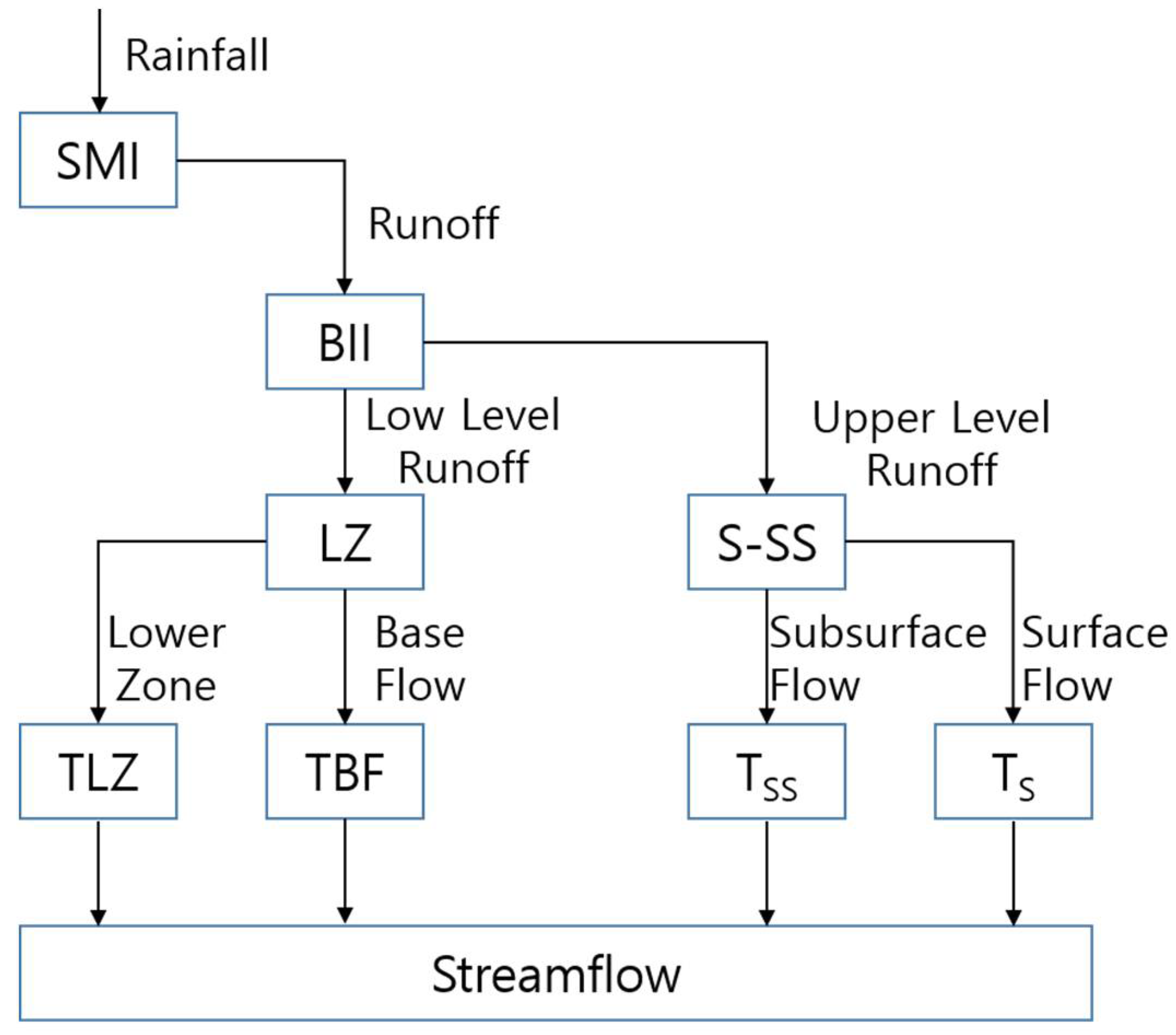
The SSARR model categorizes runoff into above-surface runoff, below-surface runoff, underwater runoff, and return underwater runoff. Assuming that each runoff consists of virtual linear reservoirs, reservoir routing was performed to calculate runoff. Figure 1 shows the internal flow of parameters used to calculate runoff under the SSARR model.
Some rainfall and snowfall become runoff in accordance with the Soil Moisture Index (SMI), while some are lost due to evapotranspiration. Based on the Baseflow Infiltration Index (BII), runoff is again classified into direct runoff and baseflow runoff. Direct runoff can be divided into above-surface runoff and below-surface runoff using Surface-Subsurface Separation (S-SS), and baseflow runoff into underwater runoff and return underwater runoff using Lower Zone (LZ) routing. The four types of runoff are independently calculated, and constitute the inflow in the watershed routing method. Here, Time of Lower Zone (TLZ) is the storage time required for routing of underwater runoff, Time of BaseFlow (TBF) for routing of return underwater runoff, Tss for routing of below-surface runoff, and Ts for routing of above-surface runoff. Among the internal parameters of the SSARR model, the most sensitive parameters to runoff are SMI, BII, and S-SS. The remaining parameters have relatively smaller influence on runoff [26]. To simulate runoff using the SSARR model, this study calibrated seven parameters: SMI, BII, S-SS, Tss, Ts, n1, and n2. Ts and Tss are storage times, and n1 and n2 are the number of virtual reservoirs. The characteristics of key parameters are as follows:
- Soil Moisture Index (SMI)
SMI, one of the most sensitive parameters to runoff in the SSARR model, is used to calculate the runoff ratio based on soil moisture conditions in the watershed. It increases with rainfall or snowfall, and decreases with evapotranspiration. SMI changes over time, as shown in Formula (1):
SMI1 and SMI2 are SMI values before and after an event, MI is the moisture in the soil, RGP is the total runoff, PH is the calculation time, and ETI represents evapotranspiration.
- Baseflow Infiltration Index (BII)
BII, which divides total runoff into direct runoff and baseflow runoff, determines the baseflow runoff ratio in relation to seepage. BII changes over time, as shown in Formula (2):
BII1 and BII2 are BII values before and after an event, RG is the total runoff ratio calculated as RGP/PH, and BIITS is the storage time.
- Surface-Subsurface Separation (S-SS)
S-SS, which divides direct runoff into above-surface runoff and below-surface runoff, determines the rate of below-surface runoff in relation to changes in direct runoff rate. This parameter reflects the characteristics of short-term runoff during the flood season, and is useful when performing analysis for the purpose of flood management.
2.1.2. Channel Routing
Similar to watershed routing, channel routing also uses the routing method of continuous virtual reservoirs. While storage time is fixed in the watershed model, storage time in channel routing is expressed as shown in Formula (3), as it decreases with increasing flow. The watershed routing method is linear, whereas the channel routing method is nonlinear:
Ts is the storage time, KTS is the constant determined by the trial and error method, Q is the flow, and n is a coefficient relating the time of storage variation as a function of discharge. The range of the n parameter is between −1 and 1, n1′ is the number of phases, and T is travel time.
3. Calibration Methods
3.1. Genetic Algorithm (GA)
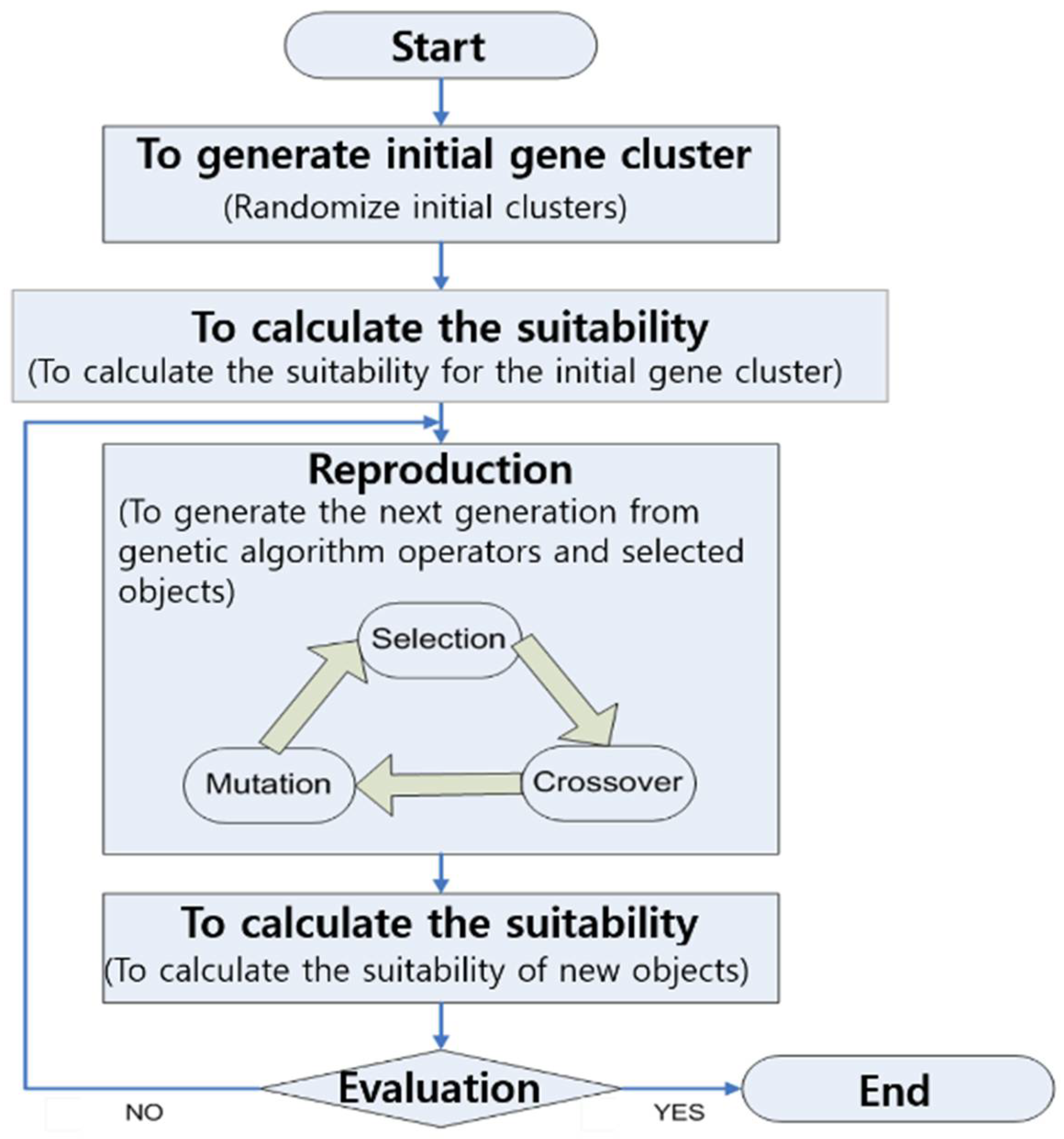
Genetic algorithm (GA), an optimization technique that simulates the concept of “survival of the fittest”, is a computational model developed, based on the adaptability of organisms to the environment and the principle of natural selection [29,30]. Since the search direction or scope relies on probabilistic differences across generations, GA is an effective optimization algorithm that is less likely to get stuck at a local minimum. The variables are selected based on objective functions to be applied to in runoff model optimization, and the initial gene cluster is generated by determining the size of genes and clusters. The adequacy of the initial cluster is calculated, which is then used to generate the next generation. The survival probability is determined using genetic operators such as selection, crossover, and mutation, and new genes are produced by switching chromosomes between two genes. The algorithm is terminated if each gene in the newly produced gene cluster satisfies the adequacy criteria, or returns to the reproduction stage if otherwise (Figure 2).
3.2. Pattern Search
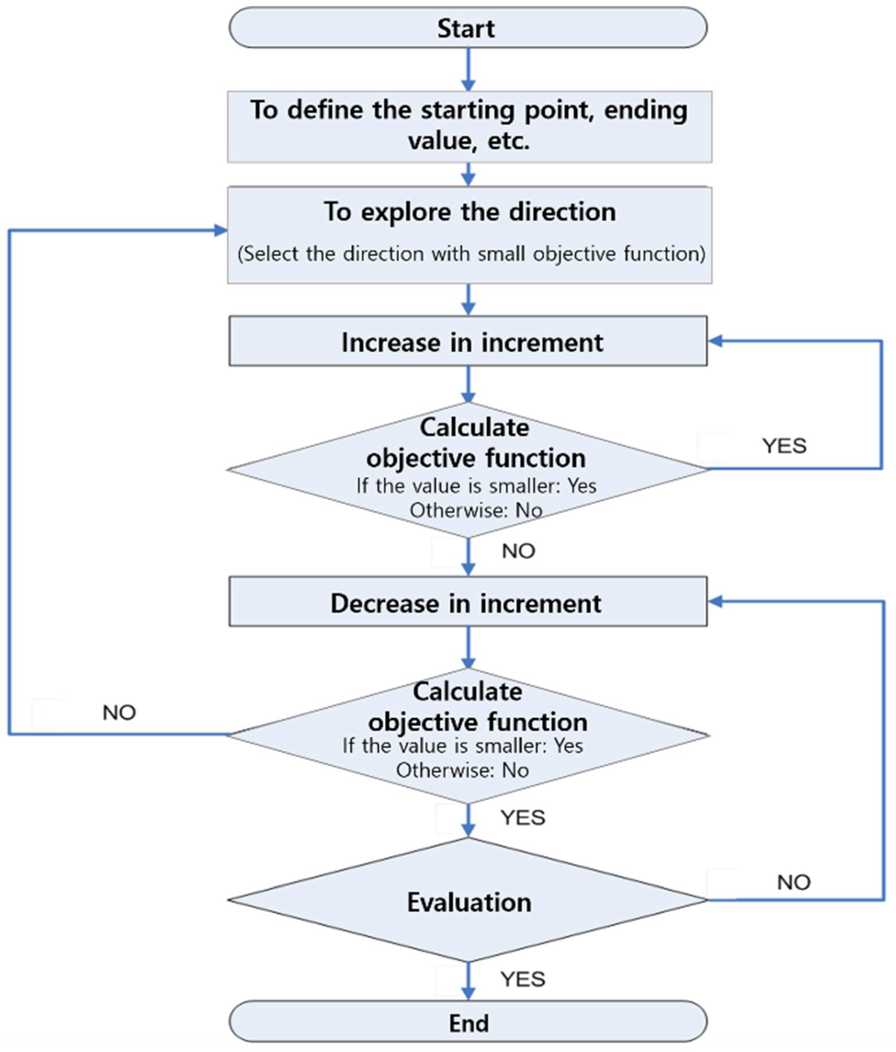
Pattern search, one of the most efficient and powerful search methods, is a direct search technique that can expand to multi-parameter functions [31,32]. From the starting point, the search heads in a direction in which the objective function grows smaller, and optimal solutions are derived by varying the increment. Formula (4) is the basic pattern search equation showing the pattern direction, size, and movement:
S11 and S21 are the starting points, and Δ is the increment. [a, b] is the direction vector, where a and b have values of −1, 0 and 1. S12 and S22 are starting points for different searches, and continue to change until the end condition is satisfied. That is, Δ and [a, b] change in a direction and size such that the objective functions of [S12, S22] become smaller. [S12, S22] is repeatedly calculated until a satisfactory objective function value is obtained or the end condition is satisfied. First, the starting point of the search, the range of possible solutions, and the end condition are determined. The objective function that is minimized is chosen among the four direction vectors ([−1, 0], [0, −1], [1, 0], [0, 1]), and the increment is increased until the objective function increases. When the objective function increases, the value obtained in the previous stage becomes the starting point, and the increment is decreased. The increment is further dropped until the objective function decreases. When the objective function decreases, the value obtained in the previous stage becomes the starting point, and the search resumes in a different direction. The pattern search method continues to vary the search direction and repeatedly increase/decrease the increment until the end condition is met or a satisfactory objective function is attained (Figure 3).
3.3. Shuffled Complex Evolution Method Developed at the University of Arizona (SCE-UA)
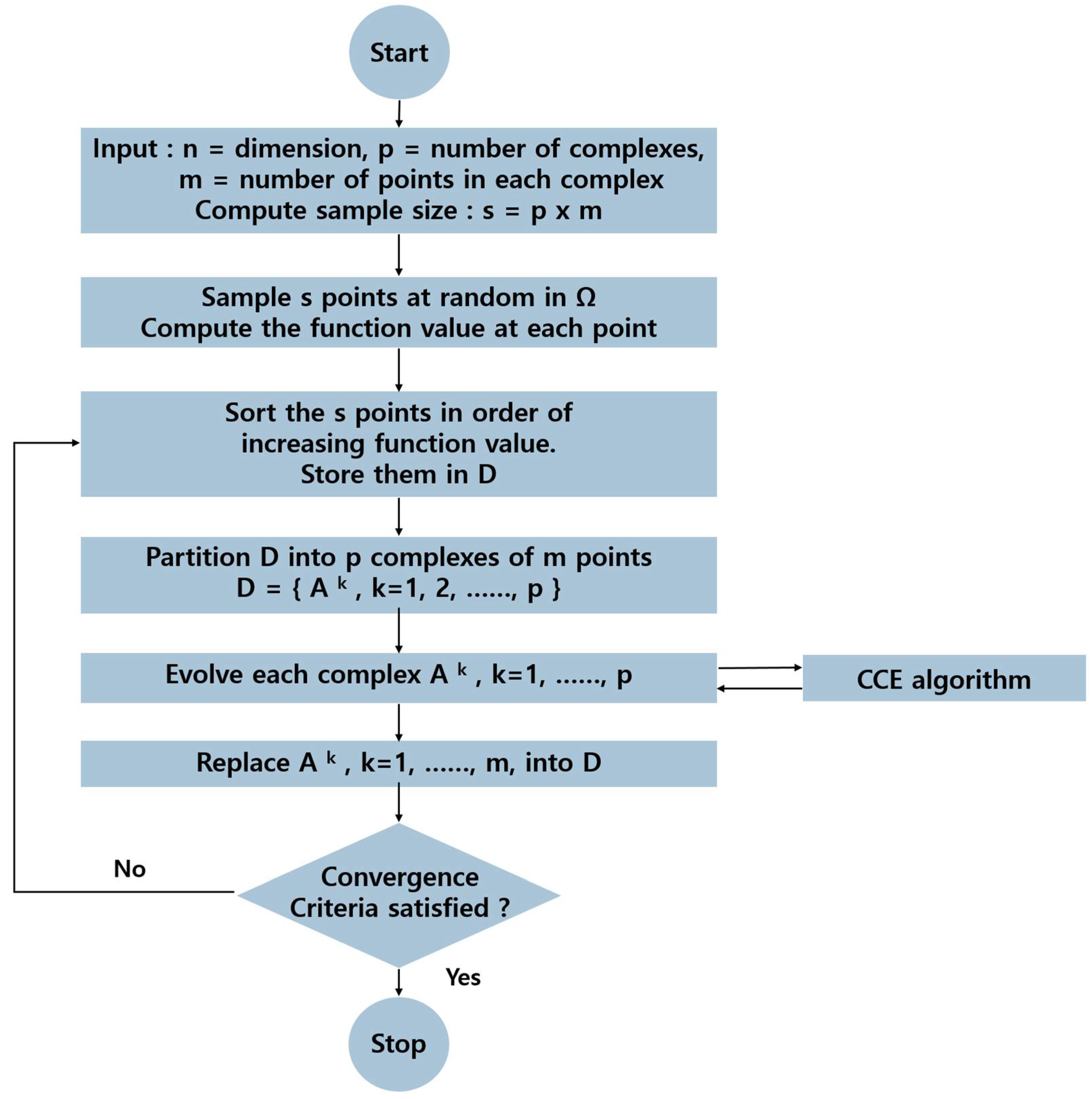
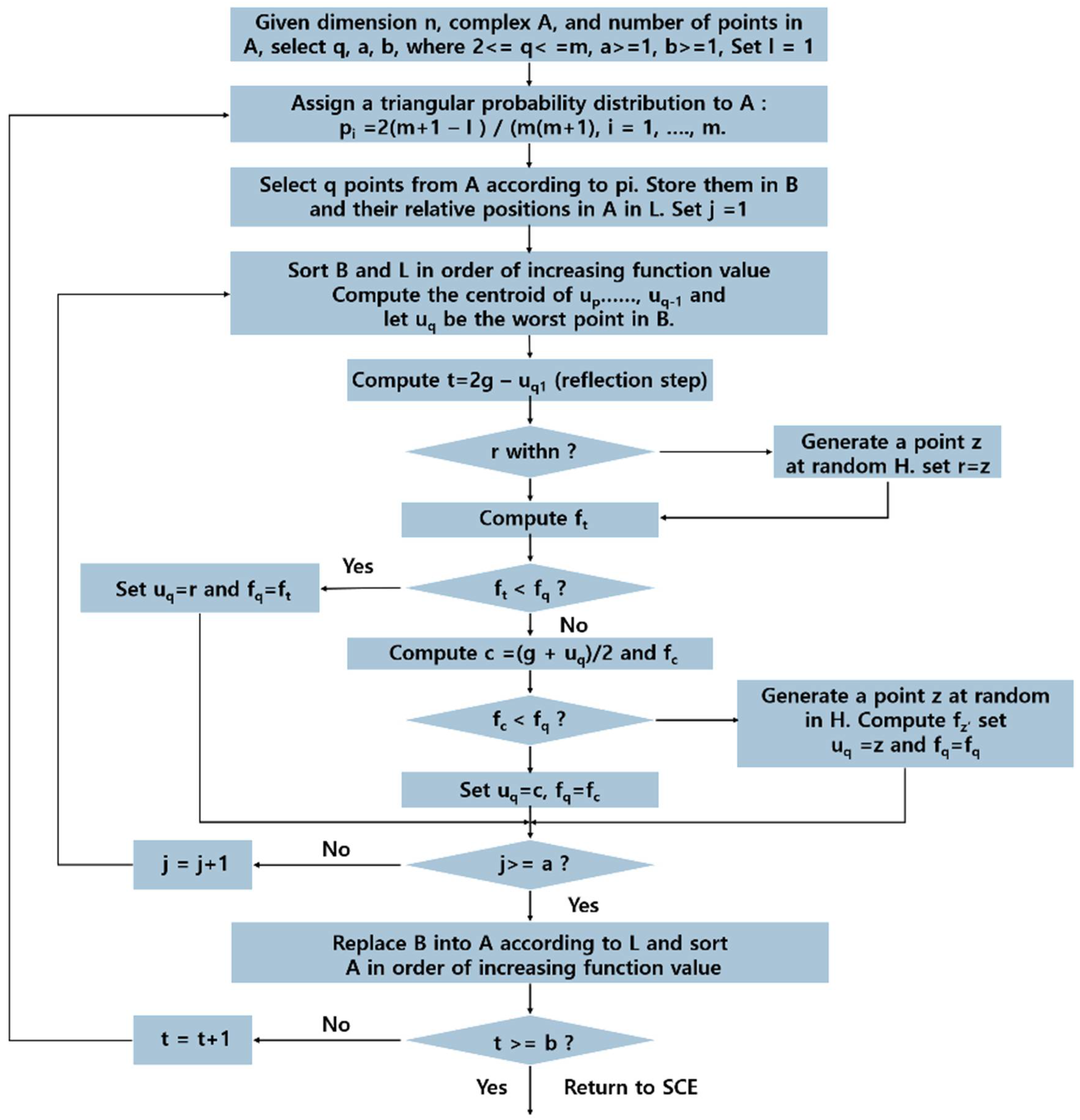
Proposed by Duan et al. [12], Shuffled Complex Evolution method developed at the University of Arizona (SCE-UA) is a global optimization procedure that combines complex shuffling with the advantages of existing search techniques such as the Simplex method [31,33], Controlled Random Search, and competitive evolution. SCE-UA effectively delivers information included in the population, and prevents the regression of such information. This characteristic makes it effective in searching for global optimal solutions in a wide range of problems [34] (Figure 4).
Through initialization, the method first determines the number of complexes (p), the number of points in a complex (m), and the number of dimensions (n). A total of s points are selected at random, and objective function values are calculated for each point. The objective functions are arranged by size. Samples are generated from p complexes, each containing m points, and each complex is evolved using the Competitive Complex Evolution (CCE) algorithm (Figure 5). The points of evolved complexes are again partitioned into p complexes, and checked for convergence. If the convergence criteria are not satisfied, the procedure is repeated from the evolution step.
4. Objective Functions
The determination of the proper objective function for parameter calibration is important for obtaining a more accurate estimate from a model.
4.1. Sum of Squared of Residual (SSR)
The objective function of Sum of Squared of Residual (SSR) is given by Formula (5), which is the sum of squared of the deviation of observed runoff and simulated runoff:
Here, n is the number of data, Qobs is the observed runoff, and Qsim is the simulated runoff. SSR commonly adopted as an objective function when performing parameter optimization for hydrologic models. Given the cumulative nature of errors, the results are highly influenced by the number of data and abnormalities. SSR is widely used for the parameter optimization of the rainfall–runoff model in flood forecasting and warning [35]. Since SSR is accumulation of error, it is influenced by the number of data and abnormal data such as high flood level. In addition, SSR does not give good results all the time for peak flow value and so we may need another objective function, which can be used for the fit of peak flow in hydrograph.
4.2. Weighted Sum of Squared of Residual (WSSR)
This study suggests an objective function called Weighted Sum of Squared of Residual (WSSR) for peak flood runoff calibration. The objective function is given by Formula (6), which assigns weights for peak flow and time of occurrence of peak flow to SSR:
i is the number of the observation, Qobs is the observed runoff, Qsim is the simulated runoff, Qobs,peak is the observed peak flow, Qsim,peak is the simulated peak flow, Tobs,peak is the time of occurrence of observed peak flow, and Tsim,peak is the time of occurrence of simulated peak flow. in WSSR is the relative error of peak flow runoff and it can be used as a weighting value for preventing overestimation and underestimation of peak flow runoff. is also the relative error of peak time and it can be used as a weighting value for diminishing lag time error. Thus, WSSR is an objective function that improves SSR for peak flow runoff and less influence of abnormal data.
5. Application to Mihocheon Stream Basin
5.1. Study Area
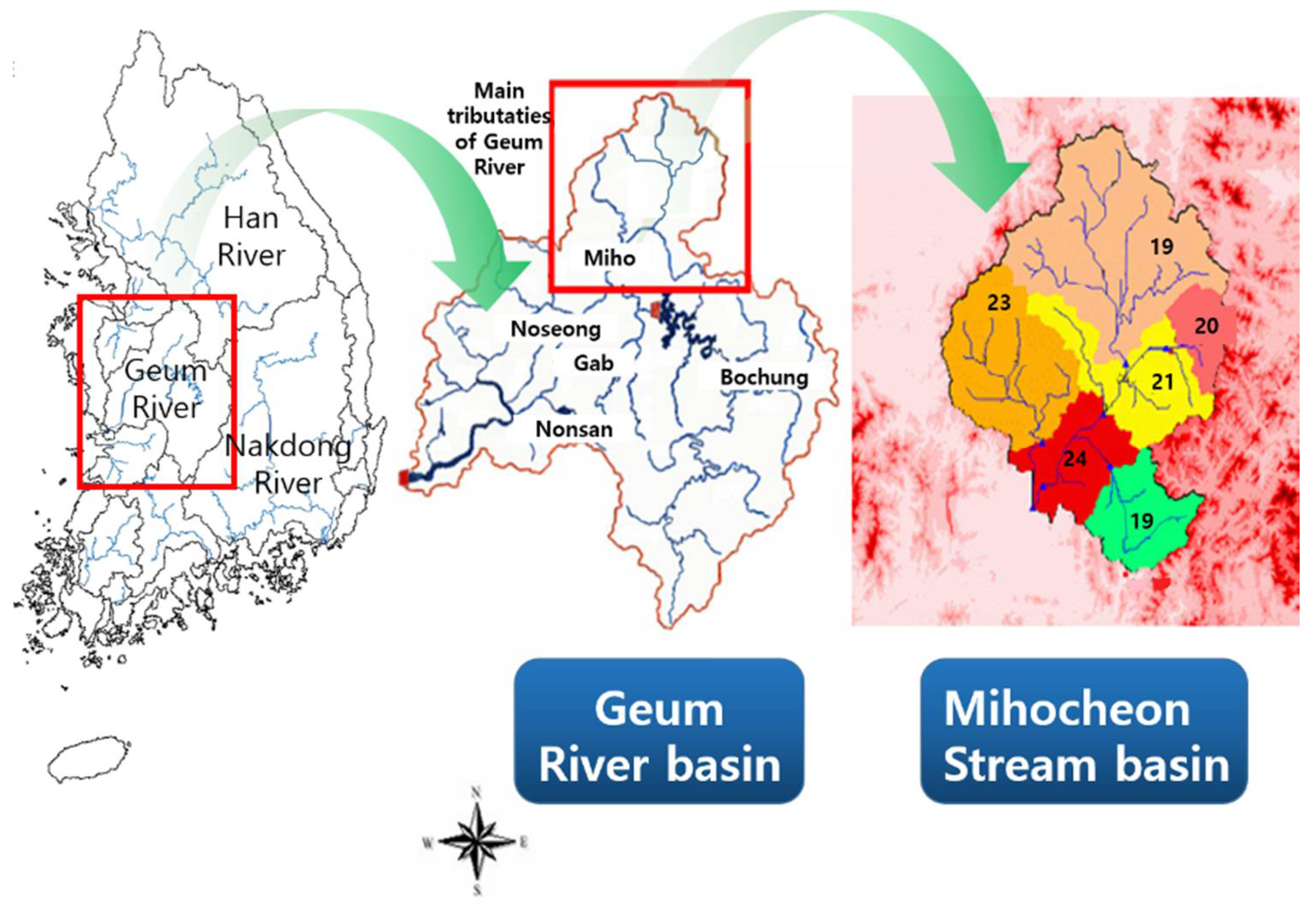
The river basin selected for analysis is the Mihocheon stream basin, located in the northern center of the Geum River basin. The Han River basin lies to the north and south of the watershed, the Anseong/Sapgyocheon stream basin to the northwest, and the Geum River basin to the south. With an area of 1850 km2, it accounts for 18.8% of the total area of the Geum River basin. Mihocheon stream has a length of 87.3 km. Sub-basins are indicated by numbers on the basin map (Figure 6). In this study, Mihocheon stream basin is divided into six sub-basins using 30 m × 30 m DEM (Digital Elevation Model) and then parameter calibration is performed after obtaining factors for basin and channel characteristics using soil map and land cover map.
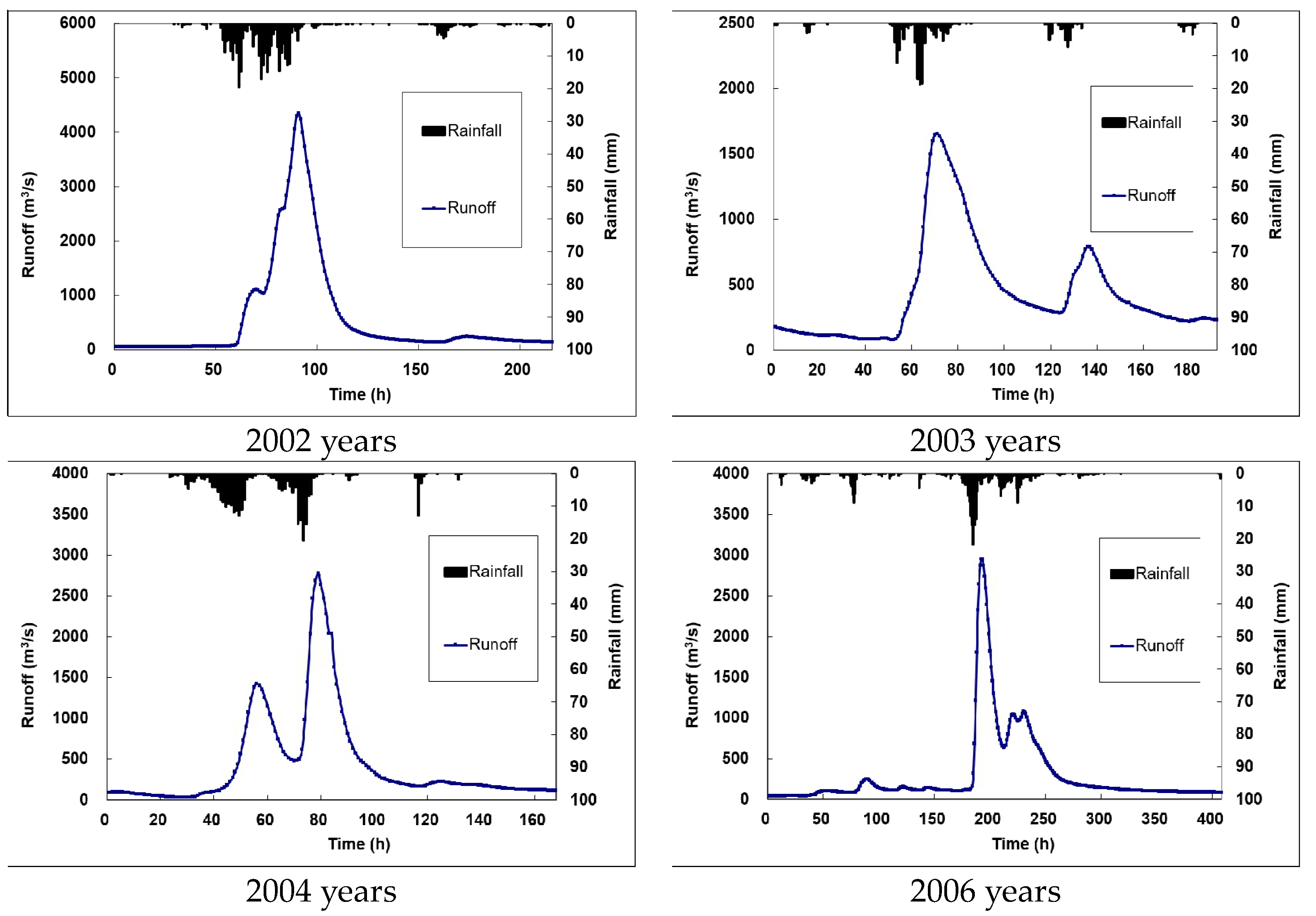
5.2. The Observed Rain Storm Events and Flood Runoff Hydrographs
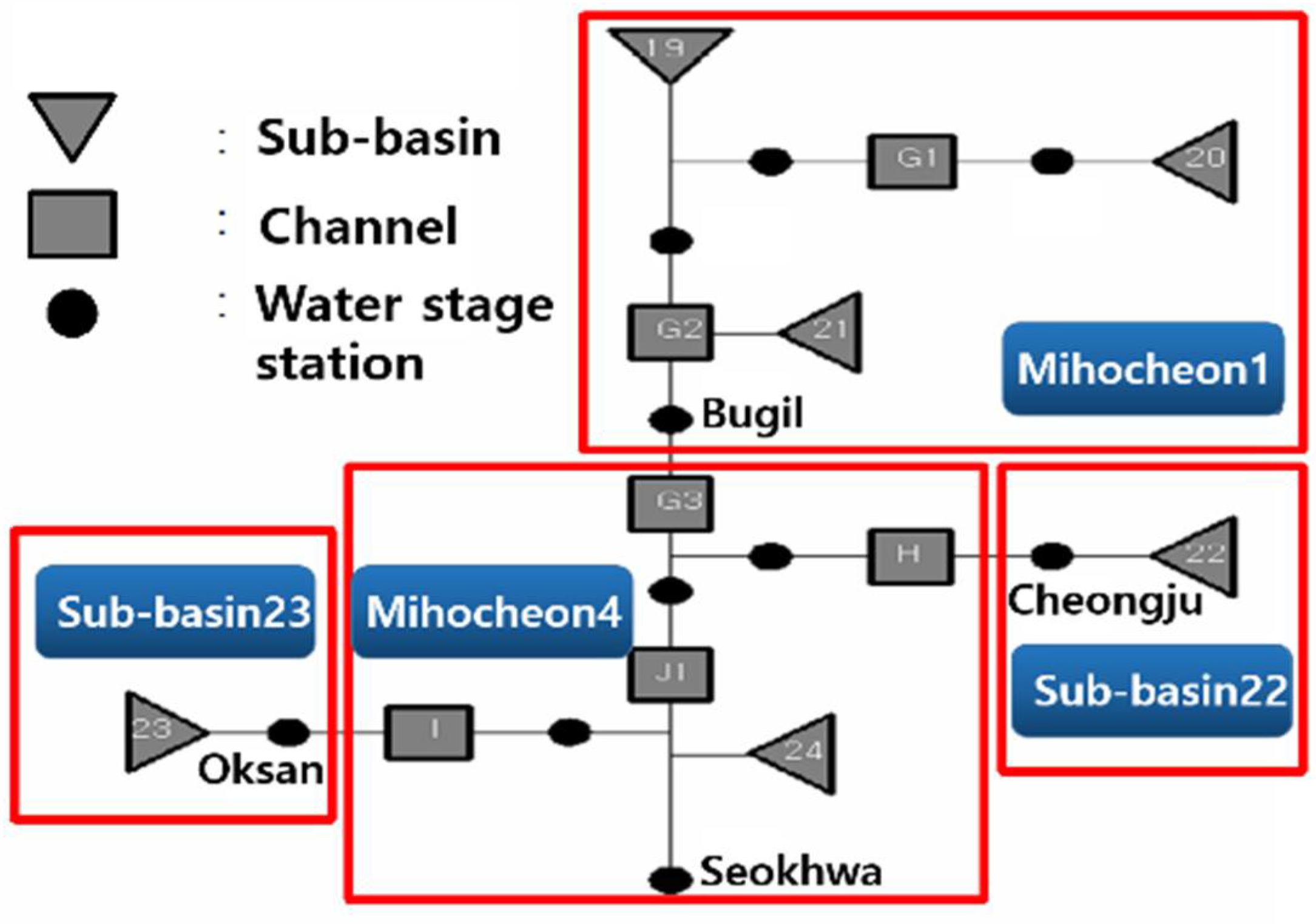
The Mihocheon stream basin is divided into six sub-basins (Sub-basin 19, Sub-basin 20, Sub-basin 21, Sub-basin 22, Sub-basin 23, Sub-basin 24) and channels (Figure 7).
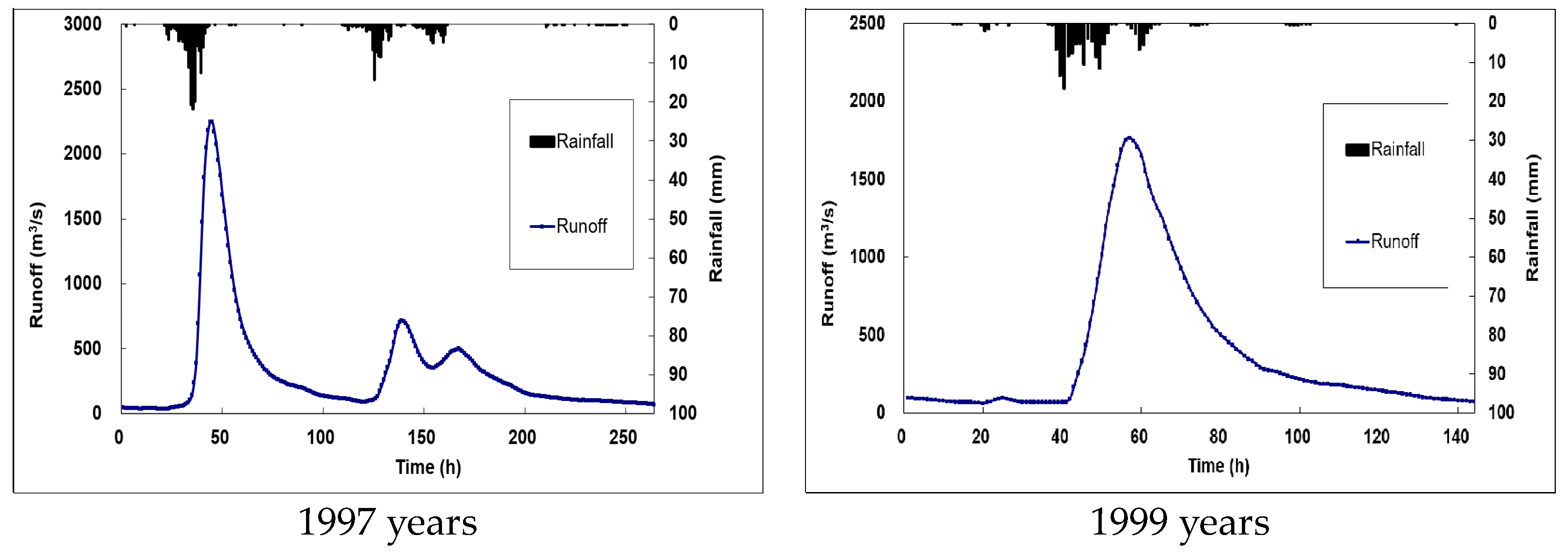
The selected rain storm events exhibited flood characteristics at all observation points in the Mihocheon stream basin and did not show extreme variation in flood runoff. Six rain storm events were selected for two sub-basins, namely Sub-basin 22 and Sub-basin 23, and calibration was performed on a total of four events that occurred between 1997 and 2003. Rain storm events dating back to 2004 and 2006 were used for validation. Table 1 shows the rain storm event data and period, while Figure 8 presents the flood runoff hydrographs of the rain storm events. Parameter calibration was performed using seven watershed parameters (SMI, BII, S-SS, Ts, Tss, n1, n2) and three channel parameters (KTS, n, n1′) of each channel.
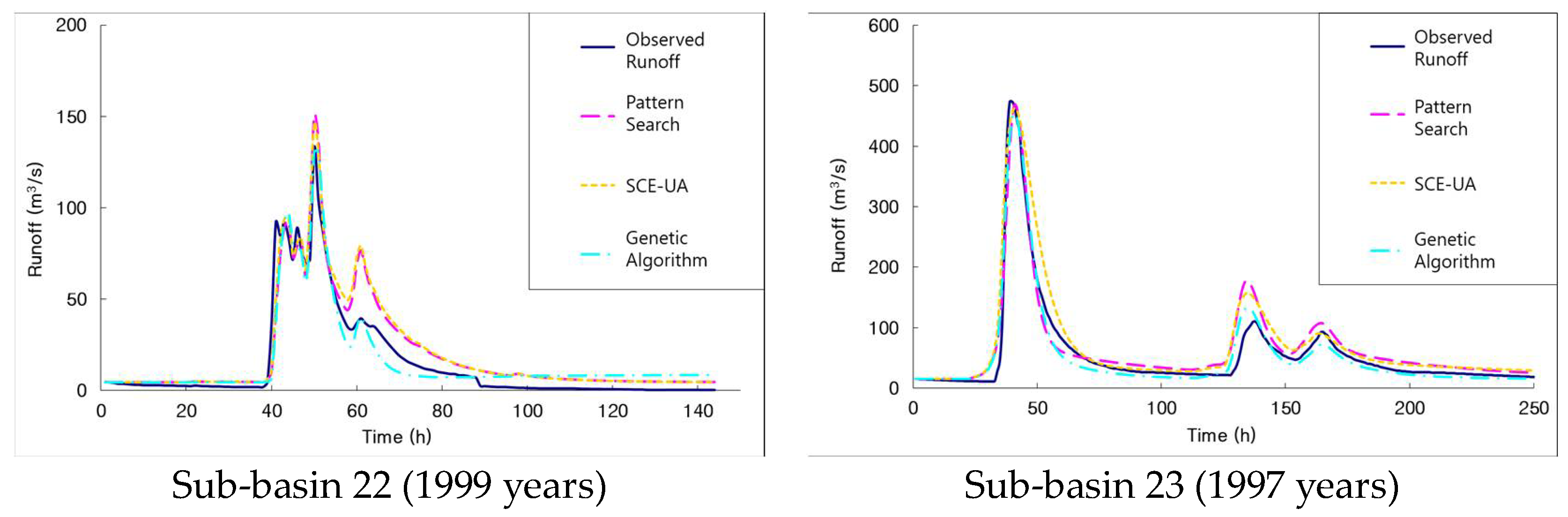
5.3. Calibration of Flood Runoff Hydrograph
Genetic algorithm has been verified as an effective method of calibration, and it was considered the most adequate calibration method in past research [36]. In addition to genetic algorithm, this study applied pattern search and SCE-UA to the calibration of parameters of the SSARR model. The evaluation criteria for calibration results consisted of the Coefficient of Determination ; Non-dimensional Root Mean Square Error (NRMSE), which is the non-dimensional form of Root Mean Square Error (RMSE) divided by observed peak flow; and Relative Error of Peak (RE), which is the difference between the observed and simulated peak flow divided by observed peak flow. The equations used as evaluation criteria are shown in Formulas (7) to (9):
i is the number of the observed data, Qobs is the observed runoff, Qsim is the simulated runoff, Qobs,peak is the observed peak flow, Qsim,peak is the simulated peak flow, Qobs,ave is the average observed runoff, and Qsim,ave is the average simulated runoff. The evaluation criteria values for each calibration method and watershed are presented in Table 2 and Table 3. And the excellent results are indicated in bold.
The calibrated flood runoff hydrographs by the above calibration methods are shown in Figure 9. Pattern search was found to be the most effective among the various calibration methods applied to the SSARR model.
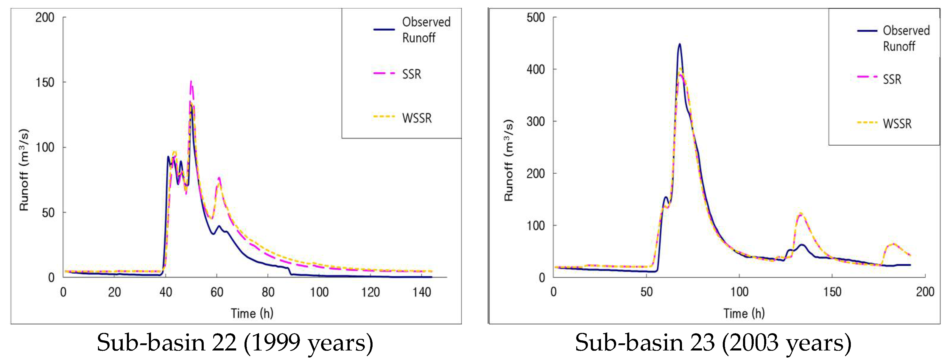
5.4. Application of WSSR Objective Function
This study assigned weights of and to obtain WSSR, and compared the results of SSR and WSSR in forecastibility for peak flood runoff. Pattern search, found to be the most effective in Section 5.3, was used for calibration. The evaluation criteria values for each objective function are presented in Table 4 and Table 5, and the calibrated flood runoff hydrographs by objective function are shown in Figure 10. And the excellent results are indicated in bold in Table 4 and Table 5.
If we compare the values obtained by evaluation criteria for SSR and WSSR in Table 4 and Table 5, we can know that WSSR is better than SRR. In addition, as shown in Figure 10, SSR produced more ideal flood runoff hydrographs, but WSSR is more accurate for peak flood runoff, which is an important element in flood forecasting. Therefore, WSSR proposed in this study, can be used more effectively for flood forecasting by the reliable estimation of peak flood runoff and lag time to peak.
6. Objective Function for Representative Parameter Estimation in a Basin
6.1. Suggestion of Objective Function for the Representative Parameter Estimation
Since the calibrated parameters of a rainfall–runoff model are usually adequate only for a studied rain storm event, we need the representative parameters which can effectively describe other rain storm events occurring in the study basin. The average values of calibrated parameters vary with rain storm events, and may not be as effective for other rain storm events. The previous study for the simulation of runoff hydrograph used an average value of different parameters according to sub-basins, but this is just proper for only one storm event used for the parameter calibration. To compensate this weakness, this study identified representative parameters of the study basin.
Four rain storm events that occurred between 1997 and 2003, were used to determine the representative parameters, which produce effective flood runoff hydrographs for various rain storm events. The method proposed in this study was to obtain parameters leading to the smallest sum of objective function values of each rain storm event. That is, parameters were estimated using an objective function that minimizes the sum of SSR for each rain storm event. The objective function is as shown in Formula (10):
Here, obj is the objective function value of SSR for each rain storm event, w is the weight of the objective function for each rain storm event, and n is the number of rain storm events. The sum of objective function values of SSR for each rain storm event becomes the basis of the proposed objective function. When calculating representative parameters, larger rain storm events have a greater influence than smaller ones on new objective functions. Weights were assigned to rain storm events such that all events have a similar influence on new objective function values.
6.2. Estimation of the Representative Parameter
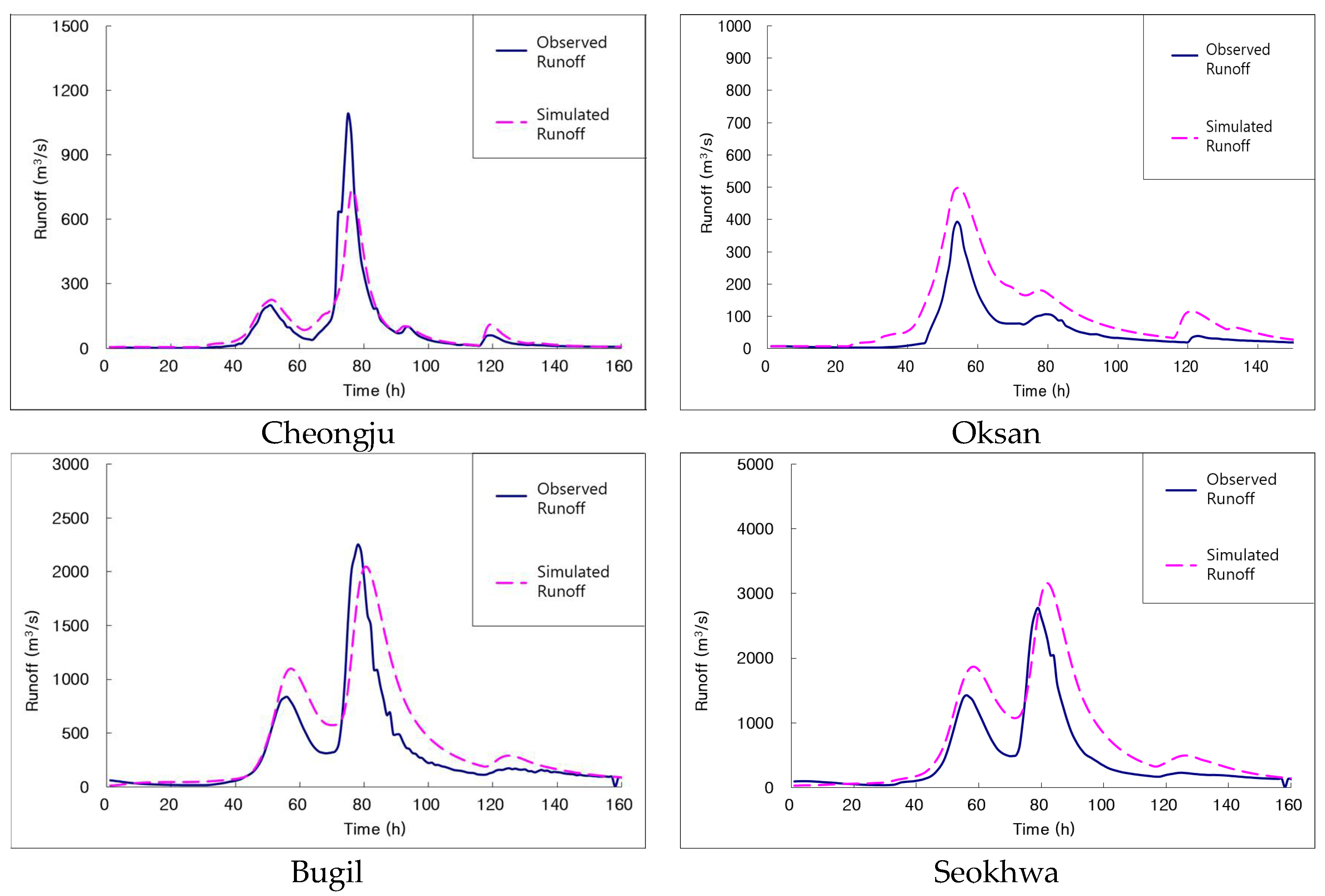
Based on the method proposed in Section 6.1, representative parameters were selected for the entire Mihocheon stream basin and applied to various rain storm events. The parameters of the rainfall–runoff model were selected from rain storm events that occurred between 1997 and 2003, and validated using rain storm events of 2004 and 2006. As shown in Table 6 and Table 7, parameters of the SSARR model for the Mihocheon stream basin were estimated according to the method proposed in Section 6.1, and a flood simulation was performed with the estimated parameters.
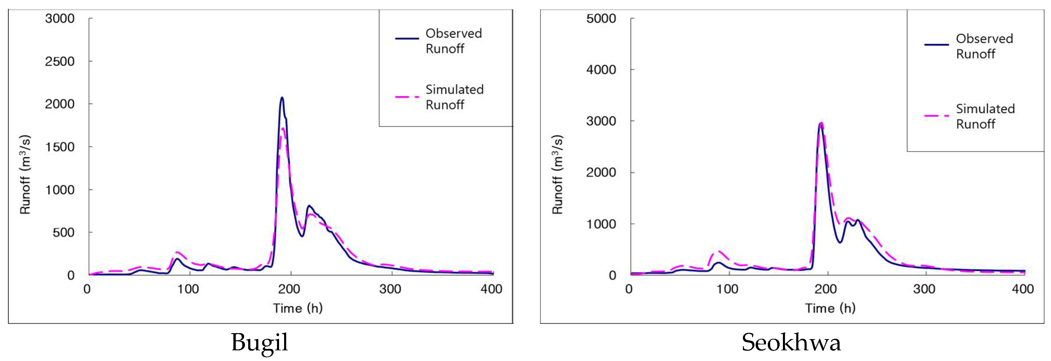
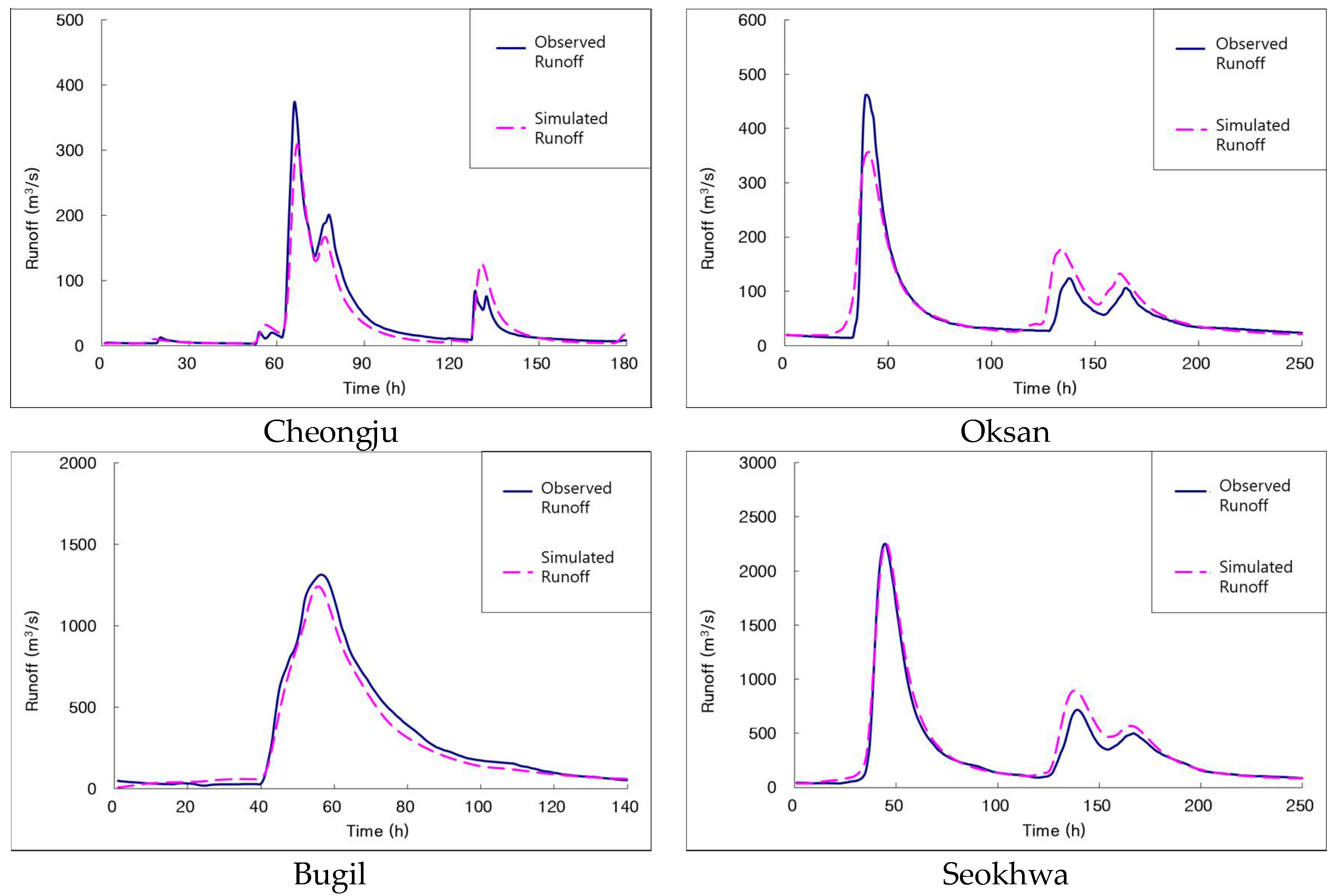
Figure 11 and Figure 12 compare the simulation results to the observed flow at each water stage observation station for the rain storm events of 2004 and 2006, respectively.
Mihocheon stream basin has its own parameters calibrated by rain storm events occurred in each year of 2004 and 2006. The validation results using the representative and basin’s own parameters for 2004 and 2006 rain storm events are expressed as evaluation criteria values in Table 8 and Table 9. If we compare the values of evaluation criteria, we can know that the representative parameter is showing more better results.
The graph of Figure 13 is the result of applying representative parameters to water stage observation stations in the basin. For the rain storm event, the results obtained at the Seokhwa water stage station was highly ideal, indicating that the representative parameters can be realistically applied to enhance the accuracy of flood forecasting and warning in the Mihocheon stream basin.
The representative parameters were found to be effective in simulating rain storm events at each water stage observation station. While parameters were limited to a single rain storm event before this study, the proposed representative parameters can be applied to several rain storm events as verified above. The use of representative parameters applicable to various rain storm events will allow flood forecasting to be faster and more accurate. The accuracy of representative parameters can be improved through application to various rain storm events.
7. Discussion
The difference between observed and simulated hydrographs by rainfall–runoff models could occur from the uncertainties from input data, measured data, non-optimized parameters, and incomplete model structure. However, only non-optimized parameters can be controlled in model calibration, and the optimized parameter set should be found by the algorithms or manual way. The objective function, as the estimation criteria of optimization algorithms, might be defined and it has been focused on the inconsistency between observed and simulated runoff hydrographs. Therefore, it has been mostly used for the fit of observed and simulated hydrographs; in this sense, SRR is widely used as the objective function. There are also other objective functions such as Proportional Error of Estimate (PEE) and Nash–Sutcliffe (NS) coefficient, but those are to fit the simulated runoff to observed runoff either, in other words, focused on observations. However, the peak flow and peak time or lag time to peak flow should be well fitted rather than overall fit of observed and simulated hydrographs for flood simulation or forecasting purpose, and the proper objective function for flood hydrographs should be used. Therefore, this study suggested WSSR for the purposes for the fit of peak flow and peak time in flood runoff hydrograph. For example, WSSR was developed using the weights from the relative errors of peak flow and peak time and can prevent the overestimation and underestimation of peak variables.
The previous studies tried to fit the observed and simulated hydrographs using the calibrated parameters of a rainfall–runoff model. However, one storm event or the specific storm events were used for model calibration, and, therefore, if the events having different characteristics occur, the calibrated parameters by previous events will not be adequate for new events. That is, the newly calibrated parameters using new events should be obtained for the runoff simulation. Therefore, this study suggested the representative parameters that can describe the same runoff characteristics for the previous and new events. To do this, the representative objective function was proposed and the representative parameters of the basin can be obtained by using this objective function. One SSR value is obtained from one event. The sum of SSR values from various rain storm events is the basic representative objective function; however, we have to say that one big event cannot have a big influence on the representative objective function. For example, if SSR of an event (E1) is 10,000 units and another (E2) is 100 units, we mostly calibrated the E1 event for minimizing the representative objective function in the calculation process. In this case, the calibration could be performed focusing on an event E1. Therefore, we have to prevent the biased calibration for one event. For this, the weights were estimated based on the peak flood runoff from each rain storm event. And, each event had the same influence on the representative objective function value.
8. Conclusions
This study applied three calibration methods, namely, genetic algorithm, pattern search, and SCE-UA, to the SSARR model, and compared runoff simulation results using two objective functions, SSR and WSSR. Representative parameters were proposed to overcome the inapplicability of estimated parameters from a single rain storm event to other rain storm events. The results derived from applying the three calibration methods (genetic algorithm, pattern search, SCE-UA) to the SSARR model are as follows. In the simulation of rain storm events, the results were more ideal when calibration was performed with a genetic algorithm and pattern search. The results were the least desirable when using SCE-UA for calibration. SCE-UA was the fastest method, and a genetic algorithm was the most time-consuming. In terms of accuracy and calculation time, the pattern search was found to be the most efficient for flood forecasting. A comparison of the objective function of SSR and WSSR showed that the latter was more accurate for peak flood runoff, which is an important element in flood forecasting. However, the objective function of SSR produced better results for runoff capacity and observed/simulated runoff hydrographs. In order to establish effective preventive measures against floods, it is more important to enhance the accuracy of peak flood runoff forecasting and the reliability of flood forecasting using the objective function of WSSR. This study proposed a method of selecting representative parameters for application to various rain storm events. Representative parameters were selected using the proposed method, and applied to rain storm events dating back to 2004 and 2006. When the representative parameters were applied to various rain storm events, this study succeeded in obtaining ideal, calibrated simulated runoff hydrographs, thereby overcoming the inapplicability of estimated parameters from a single rain storm event to other rain storm events. The results demonstrate the usefulness of representative parameters, and further improvements to the accuracy and reliability of flood forecasting can be expected from selecting representative parameters based on various rain storm events.
Author Contributions
This research was carried out in collaboration among all authors. H.S.K. had the original idea and led the research; J.K., D.K., H.J., H.N. and J.L. performed the data processing and analysis; and J.K. and J.L. edited the final manuscript. All authors reviewed and approved the manuscript.
Funding
This research was funded by the Korea Agency for Infrastructure Technology Advancement (KAIA) grant funded by the Ministry of Land, Infrastructure and Transport (Grant 18AWMP-B083066-05).
Acknowledgments
This work is supported by the Korea Agency for Infrastructure Technology Advancement (KAIA) grant funded by the Ministry of Land, Infrastructure and Transport (Grant 18AWMP-B083066-05). This work was supported by the National Research Foundation of Korea (NRF) grant funded by the Korea government (MSIT) (No. 2017R1A2B3005695).
Conflicts of Interest
The authors declare no conflict of interest.
References
- Kim, B.J.; Kwak, J.W.; Lee, J.H.; Kim, H.S. Calibration and estimation of parameter for storage function model. J. Korean Soc. Civ. Eng. 2008, 28, 21–32. [Google Scholar]
- Kim, D.H.; Hong, S.J.; Han, D.G.; Choi, C.H.; Kim, H.S. Analysis of future meteorological drought index considering climate change in Han-River Basin. J. Wetl. Res. 2016, 18, 432–447. [Google Scholar] [CrossRef]
- Brocca, L.; Melone, F.; Moramarco, T. Distributed rainfall–runoff modelling for flood frequency estimation and flood forecasting. Hydrol. Process. 2011, 25, 2801–2813. [Google Scholar] [CrossRef]
- Cundy, T.W.; Brooks, K.N. Calibrating and verifying the SSARR model, Missouri river watersheds study. J. Am. Water Resour. Assoc. 1981, 17, 775–782. [Google Scholar] [CrossRef]
- Environment Canada. Hydrotechnical Study of the Steady Brook Area, Main Report; Canada-Newfoundland Flood Damage Reduction Program St. John’s NF: St. John’s, NL, Canada, 1984.
- Picco, R.A. Comparative Study of Flow Forecasting in the Humber River Basin Using a Deterministic Hydrologic Model and a Dynamic Regression Statistical Model. Master’s Thesis, Memorial University of Newfoundland, St. John’s, NL, Canada, 1997. [Google Scholar]
- Shahzad, M.K. A Data Based Flood Forecasting Model for the Mekong River. Ph.D. Thesis, Karlsruhe Institute of Technology, Karlsruhe, Baden-Württemberg, Germany, 2011. [Google Scholar]
- Lee, S.J.; Maeng, S.J.; Kim, H.S.; Na, S.I. Analysis of runoff in the Han River basin by SSARR model considering agricultural water. Paddy Water Environ. 2012, 10, 265–280. [Google Scholar] [CrossRef]
- Victor, P.; Alexander, P. Evaluating a Hydrological Flood Routing Function for Implementation into a Hydrological Energy Model. Master’s Thesis, Lund University, Lund, Sweden, 2012. [Google Scholar]
- Kim, H.S.; Muhammad, A.; Maeng, S.J. Hydrologic Modeling for Simulation of Rainfall-Runoff at Major Control Points of Geum River Watershed. Procedia Eng. 2016, 154, 504–512. [Google Scholar] [CrossRef]
- Valeo, C.; Xiang, Z.; Bouchart, J.C.; Yeung, P.; Ryan, M.C. Climate Change Impacts in the Elbow River Watershed. Can. Water Resour. J. 2007, 32, 285–302. [Google Scholar] [CrossRef]
- Duan, Q.; Sorooshian, S.; Gupta, V.K. Effective and efficient global optimization for conceptual rainfall–runoff models. Water Resour. Res. 1992, 28, 1015–1031. [Google Scholar] [CrossRef]
- Duan, Q.; Sorooshian, S.; Gupta, V.K. Optimal use of the SCE-UA global optimization method for calibrating watershed models. J. Hydrol. 1994, 158, 265–284. [Google Scholar] [CrossRef]
- Gan, T.Y.; Biftu, G.F. Automatic calibration of conceptual rainfall–runoff models: Optimization algorithms, catchment conditions and model structure. Water Resour. Res. 1996, 32, 3513–3524. [Google Scholar] [CrossRef]
- Cheng, C.T.; Ou, C.P.; Chau, K.W. Combining a fuzzy optimal model with a genetic algorithm to solve multi-objective rainfall–runoff model calibration. J. Hydrol. 2002, 268, 72–86. [Google Scholar] [CrossRef]
- Hay, L.E.; Leavesley, G.H.; Clark, M.P.; Markstrom, S.L.; Viger, R.J.; Umemoto, M. Step wise, multiple objective calibration of a hydrologic model for a snowmelt dominated basin. J. Am. Water Resour. Assoc. 2006, 42, 877–890. [Google Scholar] [CrossRef]
- Zhang, C.; Wang, R.; Meng, Q. Calibration of Conceptual Rainfall-Runoff Models Using Grobal Optimization. Adv. Meteorol. 2015, 2015, 1–12. [Google Scholar]
- Rode, M.; Arhonditsis, G.; Balin, D.; Kebede, T.; Krysanova, V.; Griensven, A.; Zee, S. New challenges in integrated water quality modeling. Hydrol. Process. 2010, 24, 3447–3461. [Google Scholar] [CrossRef]
- Grimaldi, S.; Petroselli, A.; Nardi, F. A parsimonious geomorphological unit hydrograph for rainfall–runoff modelling in small ungauged basins. Hydrol. Sci. J. 2012, 57, 73–83. [Google Scholar] [CrossRef]
- Uusitalo, L.; Lehikoinen, A.; Helle, I.; Myrberg, K. An overview of methods to evaluate uncertainty of deterministic models in decision support. Environ. Model. Softw. 2015, 63, 24–31. [Google Scholar] [CrossRef]
- Palomba, F.; Cesari, G.; Pelillo, R.; Petroselli, A. An empirical model for river ecological management with uncertainty evaluation. Water Resour. Manag. 2017, 32, 897–912. [Google Scholar] [CrossRef]
- Chen, Y.; Xu, H. Improving flood forecasting capability of physically based distributed hydrological models by parameter optimization. Hydrol. Earth Syst. Sci. 2016, 20, 375–392. [Google Scholar] [CrossRef]
- Huo, J.; Zhang, Y.; Luo, L.; Long, Y.; He, Z. Model parameter optimization method research in Heihe River open modeling environment (HOME). J. Pattern Recognit. Artif. Intell. 2017, 31, 31–53. [Google Scholar] [CrossRef]
- Kouchi, D.H.; Esmaili, K.; Faridhosseini, A.; Sanaeinejad, S.H.; Khalili, D.; Abbaspour, K.C. Sensitivity of Calibrated Parameters and Water Resource Estimates on Different Objective Functions and Optimization Algorithms. Water 2017, 9, 384. [Google Scholar] [CrossRef]
- Rockwood, D.M. User Manual for COSSARR Model: A Digital Computer Program Designed for Small to Medium Scale Computers for Performing Streamflow Synthesis and Reservoir Regulation in Conversational Model; US Engineer Division, North Pacific: Honolulu, HI, USA, 1972. [Google Scholar]
- Mastin, M.C.; Le, T. User’s Guide to SSARRMENU; US Geological Survey, Open-File Report 01-439; Charles G. Groat: Tacoma, WA, USA, 2002.
- Cai, H. Flood Forecasting on the Humber River Using an Artificial Neural Network Approach. Master’s Thesis, Memorial University of Newfoundland, St. John’s, NL, Canada, 2010. [Google Scholar]
- USACE. SSARR Users Manual; North Pacific Division: Portland, OR, USA, 1987. [Google Scholar]
- Civicioglu, P. Transforming Geocentric Cartesian Coordinates to Geodetic Coordinates by Using Differential Search Algorithm. Comput. Geosci. 2012, 46, 229–247. [Google Scholar] [CrossRef]
- Patrascu, M.; Stancu, A.F.; Pop, F. HELGA: A heterogeneous encoding lifelike genetic algorithm for population evolution modeling and simulation. Soft Comput. 2014, 18, 2565–2576. [Google Scholar] [CrossRef]
- McKinnon, K.I.M. Convergence of the Nelder—Mead simplex method to a non-stationary point. SIAM J. Optim. 1999, 9, 148–158. [Google Scholar] [CrossRef]
- Dolan, E.D.; Lewis, R.M.; Torczon, V.J. On the local convergence of pattern search (PDF). SIAM J. Optim. 2003, 14, 567–583. [Google Scholar] [CrossRef]
- Powell, M.J.D. On Search Directions for Minimization Algorithms. Math. Program. 1973, 4, 193–201. [Google Scholar] [CrossRef]
- Jeon, J.H.; Park, C.G.; Engel, B.A. Comparison of Performance between Genetic Algorithm and SCE-UA for Calibration of SCS-CN Surface Runoff Simulation. Water 2014, 6, 3433–3456. [Google Scholar] [CrossRef]
- Diskin, M.H.; Simon, E. A procedure for the selection of objective functions for hydrologic simulation models. J. Hydrol. 1977, 34, 129–149. [Google Scholar] [CrossRef]
- Song, J.H.; Kim, H.S.; Hong, I.P.; Kim, S.Y. Parameter calibration of storage function model and flood forecasting (1) calibration methods and evaluation of simulated flood hydrograph. J. Korean Soc. Civ. Eng. 2006, 26, 27–38. [Google Scholar]
Figure 1.
Parameters and runoffs in the SSARR model.

Figure 2.
Flowchart of genetic algorithm.

Figure 3.
Flowchart of pattern search.

Figure 4.
Flowchart of the SCE-UA algorithm.

Figure 5.
CCE algorithm of SCE-UA.

Figure 6.
Sub-basins in the Mihocheon stream basin.

Figure 7.
Schematic diagram of channel and water stage stations in the Mihocheon stream basin.

Figure 8.
Rain storm events and runoff hydrographs used.


Figure 9.
Comparison of observed and calibrated runoff hydrographs.

Figure 10.
Comparison of the observed and simulated runoff hydrographs by SSR and WSSR.

Figure 11.
The observed and simulated runoff hydrographs for verification in each water stage station (for rain event of 2004).
Figure 11.
The observed and simulated runoff hydrographs for verification in each water stage station (for rain event of 2004).

Figure 12.
The observed and simulated runoff hydrographs for verification in each water stage station (for rain event of 2006).
Figure 12.
The observed and simulated runoff hydrographs for verification in each water stage station (for rain event of 2006).


Figure 13.
The simulated runoff hydrographs by the estimated representative parameters.


Table 1.
Rain storm events and flood runoff hydrographs used.
| Classification | Data Period |
|---|---|
| Calibration Event | 30 June 1997–10 July 1997 |
| 1 August 1999–6 August 1999 | |
| 4 August 2002–12 August 2002 | |
| 20 July 2003–27 July 2003 | |
| Validation Event | 18 June 2004–24 June 2004 |
| 9 July 2006–25 July 2006 |
Table 2.
The values of evaluation criteria for calibration methods in Sub-basin 22.
| Objective Functions | Year of Rain Storm Events | Evaluation Criteria | Calibration Methods | ||
|---|---|---|---|---|---|
| GA | Pattern Search | SCE-UA | |||
| SSR | 1997 | R2 | 0.9655 | 0.9633 | 0.9638 |
| NRMSE | 0.0375 | 0.0367 | 0.0412 | ||
| RE | 0.0008 | 0.0005 | 0.0614 | ||
| 1999 | R2 | 0.8989 | 0.9070 | 0.9131 | |
| NRMSE | 0.0649 | 0.0667 | 0.0709 | ||
| RE | 0.0180 | 0.1309 | 0.0990 | ||
| 2002 | R2 | 0.9288 | 0.9337 | 0.8854 | |
| NRMSE | 0.0644 | 0.0610 | 0.0781 | ||
| RE | 0.1744 | 0.1645 | 0.0073 | ||
| 2003 | R2 | 0.9606 | 0.9606 | 0.9303 | |
| NRMSE | 0.0408 | 0.0385 | 0.0513 | ||
| RE | 0.1071 | 0.1039 | 0.1492 | ||
Table 3.
The values of evaluation criteria for calibration methods in Sub-basin 23.
| Objective Functions | Year of Rain Storm Events | Evaluation Criteria | Calibration Methods | ||
|---|---|---|---|---|---|
| GA | Pattern Search | SCE-UA | |||
| SSR | 1997 | R2 | 0.9611 | 0.9362 | 0.9393 |
| NRMSE | 0.0344 | 0.0470 | 0.0586 | ||
| RE | 0.0402 | 0.0092 | 0.0236 | ||
| 1999 | R2 | 0.9436 | 0.9689 | 0.9231 | |
| NRMSE | 0.0639 | 0.0427 | 0.0823 | ||
| RE | 0.2278 | 0.1693 | 0.2760 | ||
| 2002 | R2 | 0.8102 | 0.7996 | 0.7655 | |
| NRMSE | 0.1487 | 0.1396 | 0.1629 | ||
| RE | 0.4553 | 0.3879 | 0.4288 | ||
| 2003 | R2 | 0.9082 | 0.9568 | 0.9335 | |
| NRMSE | 0.0772 | 0.0490 | 0.0783 | ||
| RE | 0.2497 | 0.1336 | 0.2891 | ||
Table 4.
The values of evaluation criteria for objective functions in Sub-basin 22.
| Calibration Methods | Model | Year of Rain Storm Events | Evaluation Criteria | Objective Functions | |
|---|---|---|---|---|---|
| SSR | WSSR | ||||
| Pattern Search | SSARR | 1997 | R2 | 0.9633 | 0.9552 |
| NRMSE | 0.0367 | 0.0382 | |||
| RE | 0.0005 | 0.0000 | |||
| 1999 | R2 | 0.9070 | 0.9157 | ||
| NRMSE | 0.0667 | 0.0770 | |||
| RE | 0.1309 | 0.0000 | |||
| 2002 | R2 | 0.9337 | 0.9337 | ||
| NRMSE | 0.0610 | 0.0598 | |||
| RE | 0.1645 | 0.1441 | |||
| 2003 | R2 | 0.9606 | 0.9579 | ||
| NRMSE | 0.0385 | 0.0372 | |||
| RE | 0.1039 | 0.0653 | |||
Table 5.
The values of evaluation criteria for objective functions in Sub-basin 23.
| Calibration Methods | Model | Year of Rain Storm Events | Evaluation Criteria | Objective Functions | |
|---|---|---|---|---|---|
| SSR | WSSR | ||||
| Pattern Search | SSARR | 1997 | R2 | 0.9362 | 0.9303 |
| NRMSE | 0.0470 | 0.0544 | |||
| RE | 0.0092 | 0.1070 | |||
| 1999 | R2 | 0.9689 | 0.9688 | ||
| NRMSE | 0.0427 | 0.0421 | |||
| RE | 0.1693 | 0.1574 | |||
| 2002 | R2 | 0.7996 | 0.7991 | ||
| NRMSE | 0.1396 | 0.1367 | |||
| RE | 0.3879 | 0.3727 | |||
| 2003 | R2 | 0.9568 | 0.9558 | ||
| NRMSE | 0.0490 | 0.0478 | |||
| RE | 0.1336 | 0.1054 | |||
Table 6.
The parameters of SSARR model for sub-basins in Mihocheon stream.
| Parameter | SMI | BII | S-SS | Ts | Tss | n1 | n2 | |
|---|---|---|---|---|---|---|---|---|
| Subbasin | ||||||||
| 19 | 1.00 | 1.00 | 0.50 | 3 | 17 | 2 | 1 | |
| 20 | 2.00 | 1.00 | 0.50 | 0 | 25 | 2 | 1 | |
| 21 | 2.00 | 1.00 | 0.50 | 7 | 28 | 2 | 1 | |
| 22 | 1.63 | 0.69 | 1.03 | 2 | 14 | 2 | 1 | |
| 23 | 2.78 | 0.00 | 0.50 | 4 | 23 | 2 | 1 | |
| 24 | 5.00 | 0.13 | 0.50 | 5 | 17 | 2 | 1 | |
Table 7.
The parameters of SSARR model for channels in Mihocheon stream.
| Parameter | KTS | n | n1′ | |
|---|---|---|---|---|
| Channel | ||||
| G1 | 7.00 | 0.20 | 2 | |
| G2 | 7.00 | 0.20 | 2 | |
| G3 | 29.38 | 0.83 | 1 | |
| H | 3.00 | 0.20 | 2 | |
| J1 | 5.69 | 0.20 | 2 | |
| I | 2.25 | 0.20 | 2 | |
Table 8.
The values of evaluation criteria for validation results (2004).
| Sub-Basin | Evaluation Criteria | Representative Parameter | Parameter in 2004 |
|---|---|---|---|
| Values | Values | ||
| 22 | R2 | 0.8472 | 0.8134 |
| NRMSE | 0.0953 | 0.1121 | |
| RE | 0.3272 | 0.3575 | |
| 23 | R2 | 0.9112 | 0.9646 |
| NRMSE | 0.1389 | 0.1144 | |
| RE | 0.2647 | 0.5034 |
Table 9.
The values of evaluation criteria for validation results (2006).
| Sub-Basin | Evaluation Criteria | Representative Parameter | Parameter in 2006 |
|---|---|---|---|
| Values | Values | ||
| 22 | R2 | 0.9743 | 0.8589 |
| NRMSE | 0.0236 | 0.0814 | |
| RE | 0.0859 | 0.0435 | |
| 23 | R2 | 0.9110 | 0.9290 |
| NRMSE | 0.0609 | 0.0752 | |
| RE | 0.0606 | 0.2896 |
© 2018 by the authors. Licensee MDPI, Basel, Switzerland. This article is an open access article distributed under the terms and conditions of the Creative Commons Attribution (CC BY) license (http://creativecommons.org/licenses/by/4.0/).
Share and Cite
MDPI and ACS Style
Kim, J.; Kim, D.; Joo, H.; Noh, H.; Lee, J.; Kim, H.S. Case Study: On Objective Functions for the Peak Flow Calibration and for the Representative Parameter Estimation of the Basin. Water 2018, 10, 614. https://doi.org/10.3390/w10050614
AMA Style
Kim J, Kim D, Joo H, Noh H, Lee J, Kim HS. Case Study: On Objective Functions for the Peak Flow Calibration and for the Representative Parameter Estimation of the Basin. Water. 2018; 10(5):614. https://doi.org/10.3390/w10050614
Chicago/Turabian StyleKim, Jungwook, Deokhwan Kim, Hongjun Joo, Huiseong Noh, Jongso Lee, and Hung Soo Kim. 2018. "Case Study: On Objective Functions for the Peak Flow Calibration and for the Representative Parameter Estimation of the Basin" Water 10, no. 5: 614. https://doi.org/10.3390/w10050614
Note that from the first issue of 2016, this journal uses article numbers instead of page numbers. See further details here.