Article

Evaluation of Unified Algorithms for Remote Sensing of Chlorophyll-a and Turbidity in Lake Shinji and Lake Nakaumi of Japan and the Vaal Dam Reservoir of South Africa under Eutrophic and Ultra-Turbid Conditions

1
Graduate School of Engineering, Hiroshima University, Higashihiroshima 739-8527, Japan
2
Estuary Research Center, Shimane University, Matsue 690-8504, Japan
3
Faculty of Agriculture, Tottori University, Tottori 680-8550, Japan
4
Graduate School of Science and Engineering, Shimane University, Matsue 690-8504, Japan
5
Agricultural Research Council-Institute for Soil, Climate and Water, Pretoria 0001, South Africa
6
School of Geography, Archaeology, and Environmental Studies, University of the Witwatersrand, Johannesburg 2000, South Africa
*
Author to whom correspondence should be addressed.
Water 2018, 10(5), 618; https://doi.org/10.3390/w10050618
Submission received: 19 April 2018 / Revised: 7 May 2018 / Accepted: 8 May 2018 / Published: 9 May 2018
(This article belongs to the Section Water Quality and Contamination)

Abstract

:
We evaluated unified algorithms for remote sensing of chlorophyll-a (Chla) and turbidity in eutrophic and ultra-turbid waters such as Japan’s Lake Shinji and Lake Nakaumi (SJNU) and the Vaal Dam Reservoir (VDR) in South Africa. To realize this objective, we used 38 remote sensing reflectance (Rrs), Chla and turbidity datasets collected in these waters between July 2016 and March 2017. As a result, we clarified the following items. As a unified Chla model, we obtained strong correlation (R2 = 0.7, RMSE = 2 mg m−3) using a two-band model (2-BM) and three-band model (3-BM), with Rrs(687)/Rrs(672) and [Rrs−1(687) − Rrs−1(672)] × Rrs(832). As a unified turbidity model, we obtained strong correlation (R2 = 0.7, RMSE = 260 NTU) using 2-BM and 3-BM, with Rrs(763)/Rrs(821) and Rrs(810) − [Rrs(730) + Rrs(770)]/2. When targeting the Sentinel-2 Multispectral Imager (MSI) frequency band, we focused on MSI Bands 4 and 5 (Rrs(740) and Rrs(775)) for the Chla algorithm. When optically separating SJNU and VDR data, it is effective to use the slopes of MSI Bands 3 and 4 (Rrs(560) and Rrs(665)) and the slopes of MSI Bands 7 and 9 (Rrs(775) and Rrs(865)).

1. Introduction

Fresh water on land, such as in rivers, lakes and reservoirs, accounts for about 0.01% of Earth’s water [1]; thus, protecting this resource is a vital global issue. In particular, monitoring water quality to detect turbid water and algal blooms is indispensable [2]. In this research, we focus on the waters of Japan’s Lake Shinji and Lake Nakaumi (SJNU), which are well known as brackish water zones with abundant fishery and sightseeing resources such as birds and clams. To protect these resources, water quality monitoring has been conducted at fixed points for a long time [3,4,5,6,7]. However, recent years have seen abnormal phenomena in water bodies such as cyanobacteria bloom, red tide, dysoxic bottom water and the sudden occurrence of seagrass [8,9]. We also focus on a second research site in this study, the Vaal Dam Reservoir (VDR) in South Africa, which is among the largest reservoirs in South Africa. The Vaal Dam was constructed in 1938 and plays a crucial role in supplying irrigation and industrial water to the Johannesburg metropolitan area [10,11]. For this reason, water quality has been conducted for a long time [12,13]. However, recent years have seen a further increase in the importance of water quality monitoring because of problems such as acidic mine drainage [14,15], increased water demand due to urbanization and uneven rainfall distribution caused by climate change [16]. Thus, SJNU and VDR have both similar historical backgrounds and current problems, so it is worth collaborating to improve the water quality monitoring techniques of both sites. Moreover, the current situation cannot be dealt with using conventional point source monitoring; thus, it is vital to establish technology such as remote sensing that can simultaneously monitor wide areas. Conventional water quality remote sensing relies mainly on algorithms dealing with blue and green light, but in optically-complex inland waters, the red and near-infrared parts of the spectrum are often used [17]. For example, methods such as two-band algorithms [18,19], three-band algorithms [20,21] and four-band algorithms [22,23] have been proposed to measure chlorophyll-a (Chla). For measuring turbidity (Turb) or total suspended solids (TSS), which is an indicator of turbidity, methods such as one-band algorithms [24,25] and two-band algorithms [26,27] have been proposed. Furthermore, Chla and turbidity algorithms, such as SCI (Synthetic Chlorophyll Index), which applied fluorescence line height [28] using the fluorescence band for more turbid conditions and a turbidity algorithm [29] using an 810-nm reflection peak under rich colored dissolved organic matter (CDOM) conditions, have been proposed. Several algorithms have been proposed for inland water, but a unified approach has not yet been established.
Based on the current state of satellite sensors, monitoring inland water quality using sensors such as the Moderate Resolution Imaging Spectroradiometer (MODIS) aboard the Terra and Aqua satellites, the Geostationary Ocean Color Imager (GOCI) aboard the Communication, Ocean and Meteorological Satellite and the Medium Resolution Imaging Spectrometer (MERIS) aboard the Envisat satellite, which have spatial resolutions of 500 m or better, high frequencies and high spectral resolutions, has become popular since 2000 [30,31,32]. Among these, MERIS, which operated from 2002–2012, used a 600–900 nm band to effectively monitor the quality of optically-complex inland water. Moreover, with an improved spatial resolution, continuous observation of small water bodies is possible with the same spectral performance. The Multispectral Imager (MSI) of the recent Sentnel-2A mission, which was launched in June 2015, has a 10–60-m spatial resolution, a 10-day repeat cycle and uses a 600–900-nm band that can be used for effective water quality monitoring. Additionally, high-resolution hyperspectral imagers, such as EO-1′s Hyperion (2000–2017), the Hyperspectral Imager for the Coastal Ocean (HICO) (2009–2014), which was installed on the International Space Station (ISS), and the Hyperspectral Imager Suite, which is scheduled to be operated on the ISS in 2019, also exist. Water quality monitoring for large rivers such as the Mississippi River using airborne hyperspectral sensors has been also conducted [33]. In addition to algorithms that do not depend on band position for inland waters with complex optical properties, these hyperspectral data will become important in the future.
Therefore, in this study, we evaluated recent water quality algorithms using field observation data for spectral reflectance, Chla and Turb) in SJNU and VDR under eutrophic and ultra-turbid conditions to assess algorithm stability.

2. Materials and Methods

2.1. Study Area and Field Survey

Table 1 shows the research area’s basic specifications. SJNU consists of brackish lakes located on the border between Japan’s Shimane and Tottori prefectures. The two lakes are connected by the 7.3 km-long Ohashi River and the main freshwater stream flows from the Hii River (accounting for about 90% Lake Shinji’s freshwater origin). Freshwater flows from the Hii River, through Lake Shinji and the Ohashi River into Lake Nakaumi and into the Sea of Japan via Miho Bay. The salinity of Lake Shinji and Lake Nakaumi is about 0.3% and about 10%, respectively, with Lake Nakaumi, which is close to the Sea of Japan, having a strong salinity layer developed in some places. Both lakes have an average transparency of about 1 m, with high phytoplankton and suspended solid concentrations. In addition, cyanobacteria (blue-green algae) and red tide blooms often occur in Lake Shinji and Lake Nakaumi, respectively. The SJNU catchment area’s average annual rainfall is about 1700–2300 mm.
VDR is a freshwater dam reservoir 56 km south of Johannesburg, South Africa. This dam is at the Vaal River drainage system, which has a catchment area entirely situated within South Africa. The name Vaal means gray-brown in Afrikaans, and the VDR is characterized by highly turbid water (known as ultra-turbid conditions). The VDR catchment area’s average annual rainfall is about 700 mm.
Field surveys of SJNU were carried out on 15 July and 12 September 2016, and field surveys of VDR were conducted on 12 September and 26 October 2016. To measure Chla and Turb, we used Hydrolab Data Sonde 5× instruments (Chla sensor: range = 0.03–500 mg m−3, accuracy = ±3%, resolution = 0.01 mg m−3; turbidity sensor: range = 0–3000 NTU, accuracy = 1% (<100 NTU), 3% (100–400 NTU), 5% (>400 NTU), resolution = 0.1 NTU), and an MS 720 portable spectral radiometer produced by EKO Ltd. (Guangzhou, China) (spectral range = 350–1050 nm, sampling interval = 3.3 nm) was used to measure remote sensing reflectance (Rrs). We measured spectral irradiance both immediately above the water surface and of solar radiation reflected by a ZB 6010 white board (Japan Color Research Laboratory) three times. We determined the remote sensing reflectance (sr−1) by calculating respective average reflectance and divided it by pi. The basic reflectance measurement method and Rrs transformation followed the method of Oyama et al. [34]. Mobley [35] and Tan et al. [36] point out the importance of removing sun and sky glint contained in Rrs. However, due to equipment and observation time, auxiliary observations such as sky radiance could not be conducted this time, so we did not make corrections for glint.

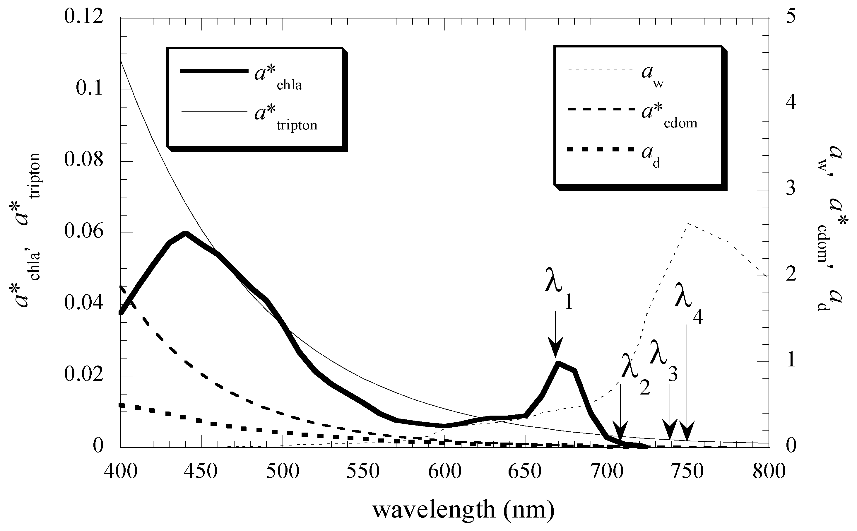
2.2. Chlorophyll-a and Turbidity Algorithms

Various remote sensing algorithms have been suggested to measure Chla and turbidity (or TSS) for inland waters with complex optical properties [17]. For example, the effectiveness of the following 2-band model (2-BM; hereinafter referred to as a C1 model) as a Chla algorithm has been shown using the red and near-infrared bands [18,19].
Chla R r s ( λ 2 ) / R r s ( λ 1 )
Recently, semi-analytical analytical models supported by the bio-optical theory have been proposed in waters that cannot be evaluated using Equation (1). For example, a 3-band model (3-BM; hereinafter referred to as a C2 model) and 4-band model (hereinafter referred to as a C3 model) [20,21,22,23] have been proposed. Here, we briefly explain these models according to bio-optical theory. Rrs observed immediately above the water surface can be expressed as:
R r s ( λ ) b b ( λ ) / [ a ( λ ) + b b ( λ ) ]
a ( λ ) = a w ( λ ) + a c d o m ( λ ) + a c h l a ( λ ) + a t r i p t o n ( λ )
b ( λ ) = b w ( λ ) + b p ( λ )
where bb is the water’s backscattering coefficient; aw, achla, acdom and atripton are the absorption coefficients of pure water, phytoplankton, CDOM and inorganic suspended matter. It is relatively easy to remotely estimate Chla in the open ocean because of the strong blue band absorption of Chla. However, Chla and CDOM from terrestrial origin both have strong blue band absorptions, making it difficult to remotely estimate Chla in inland water. Therefore, remote estimation in inland water relies on near-infrared bands, which have relatively small absorption for CDOM and similar acdom and atripton values. Only achla, which is closely related to Chla, can be extracted by removing the influence of CDOM through relatively simple arithmetic operations. Figure 1 shows absorption coefficient spectral characteristics of underwater substances and four basic wavelengths (λ1, λ2, λ3 and λ4) typically used for Chla estimation.
The C2 model calculates achla depth by taking the difference between Chla absorption’s maximum (λ1) and minimum (λ2) wavelengths, which is the reciprocal number of Rrs, and by multiplying Chla by Rrs near 740 nm, which is very small. This cancels the influence of bb in the denominator.
Chla [ R 1 ( λ 1 ) R 1 ( λ 2 ) ] [ R ( λ 3 ) ] = [ a c h l a ( λ 1 ) + a w ( λ 1 ) a w ( λ 2 ) ] / a w ( λ 3 )
However, if the absorption component of the detritus (ad) value that was omitted in Equation (3) is included, and thus cannot be ignored, Equation (5) may have a large error. Therefore, to alleviate the influence of ad by using wavelengths in which ad is assumed to have about the same range (for example, 720 nm and 750 nm), we replace R−1 (λ3) in Equation (5) with “R−1(λ4) − R−1(λ3)” to create the following 4-band model.
Chla [ R 1 ( λ 1 ) R 1 ( λ 2 ) ] [ R 1 ( λ 4 ) R 1 ( λ 3 ) ] 1 = [ a c h l a ( λ 1 ) + a w ( λ 1 ) a w ( λ 2 ) ] / [ a w ( λ 4 ) a w ( λ 3 )
Because λ3 and λ4 are close bands with similar optical characteristics, they are sometimes expressed as the following 3-BM.
Chla [ R 1 ( λ 1 ) R 1 ( λ 2 ) ] [ R 1 ( λ 4 ) R 1 ( λ 3 ) ] 1 = [ a c h l a ( λ 1 ) + a w ( λ 1 ) a w ( λ 2 ) ] / [ a w ( λ 3 ) a w ( λ 2 ) ]
In contrast, the turbidity algorithm uses an empirical single-band model (hereinafter referred to as the T1 model) [24,25] and a 2-BM (hereinafter referred to as the T2 model) [26,27] using red to near-infrared bands as follows.
Turb R r s ( λ 5 )
Turb R r s ( λ 6 ) / R r s ( λ 7 )
where Turb describes turbidity. Furthermore, in waters with a large CDOM influence, a 3-BM (hereinafter referred to as the T3 model) [29] with a high Rrs of 810 nm as an index has recently been proposed.
Turb R r s ( λ 10 ) [ R r s ( λ 9 ) + R r s ( λ 11 ) ] / 2
In this paper, we validated the basic algorithm local data and the three Chla models and three turbidity models explained so far. Table 2 summarizes these algorithms.

2.3. Accuracy Assessment

To evaluate discrepancies between the model and measured values in Table 3, we calculated the root mean square error (RMSE), which is often used to assess accuracy during water quality remote sensing algorithm evaluation [21].
R M S E = i = 1 N ( W Q p r e d , i W Q m e a s , i ) 2 N
Here, N is the number of samples; WQpred,i is the predicted value of Chla or turbidity; and WQmeas,i is the measured value of Chla or turbidity for each sample.

2.4. Simulated Satellite Data

To monitor Chla and turbidity using satellite data in the future, we simulated Rrs observed from each satellite data band using actual measurement data. Specifically, Rrs of the center wavelength for Sentinel-2 bands was extracted from the measurement Rrs data. However, because the normal Ocean Color sensor’s spatial resolution of 1 km is insufficient for monitoring on the scale of lakes and reservoirs, we used the Sentinel-2 MSI, which has a 10-m–30-m resolution. Table 3 shows MSI’s performance.

3. Results

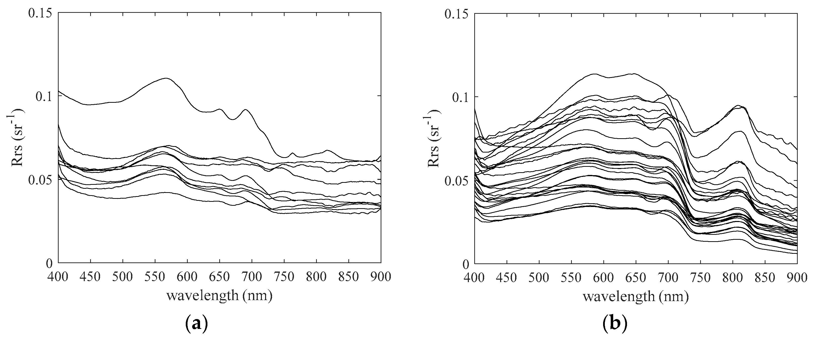
3.1. In Situ Measurements of Water Quality and Rrs

Figure 2 shows detailed sampling points (basic stationary point), and Appendix A lists all Rrs, Chla and turbidity data. Figure 3 shows the acquired spectral reflectance data. Measured Chla and turbidity data at a water depth of 0 m were used. Although SJNU and VDR had nearly identical Chla, VDR has turbidity values about 100- and 1000-times greater than SJNU, as shown in Table 4.

3.2. Algorithm Evaluation Using Field Spectra

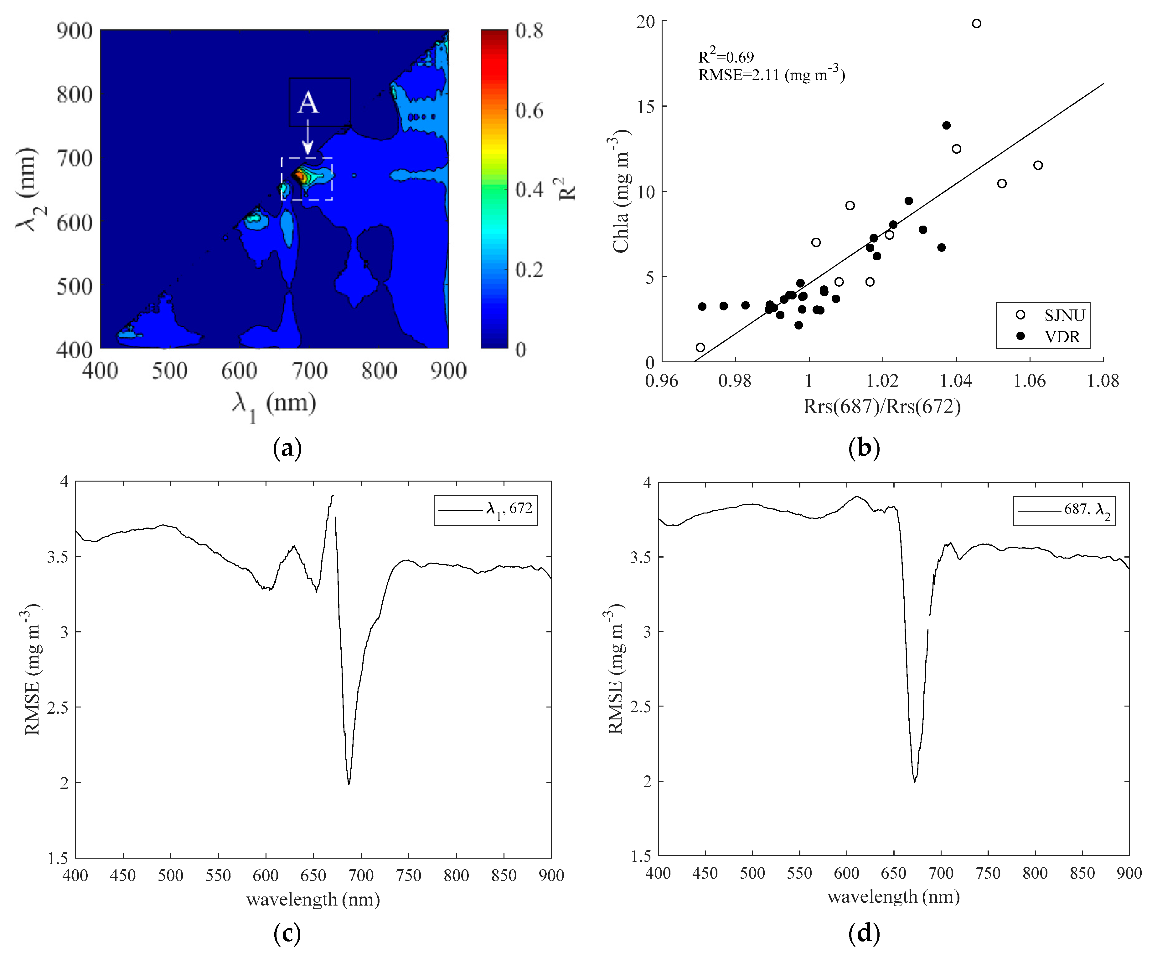
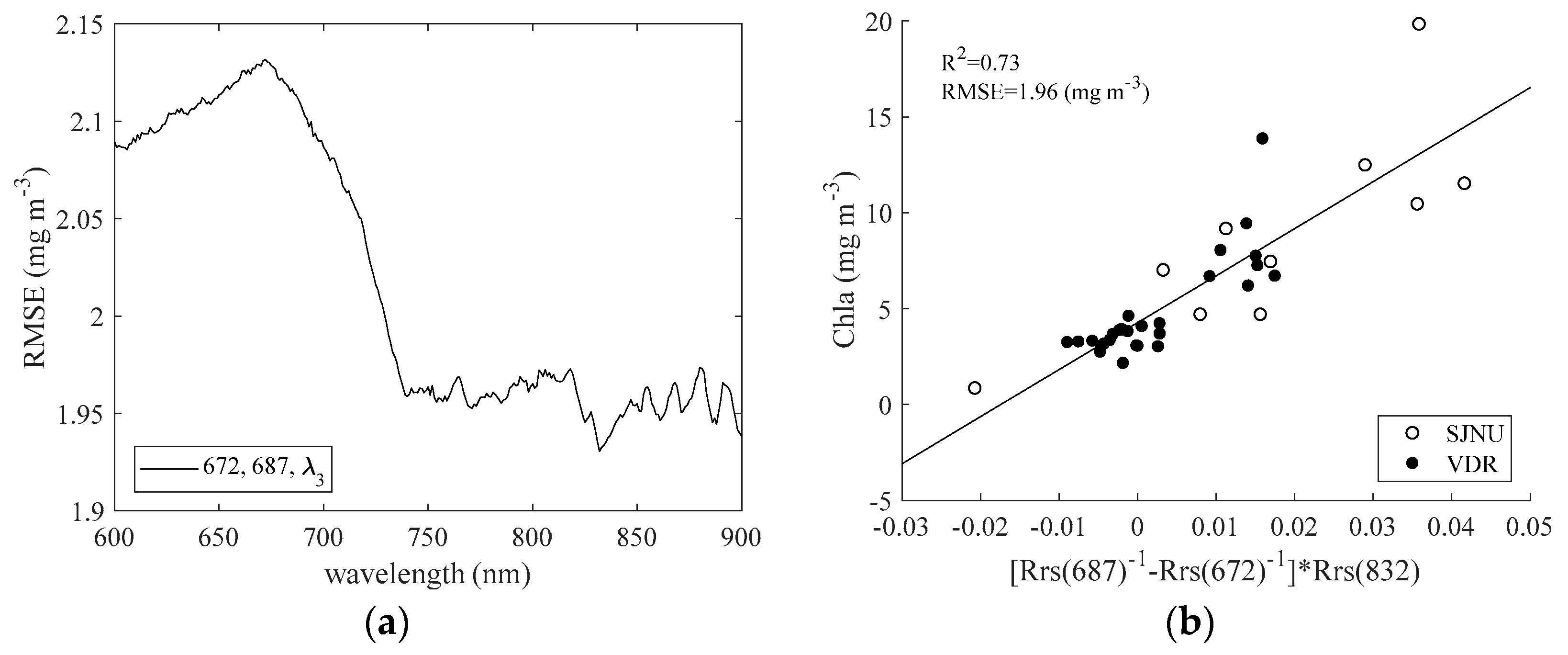
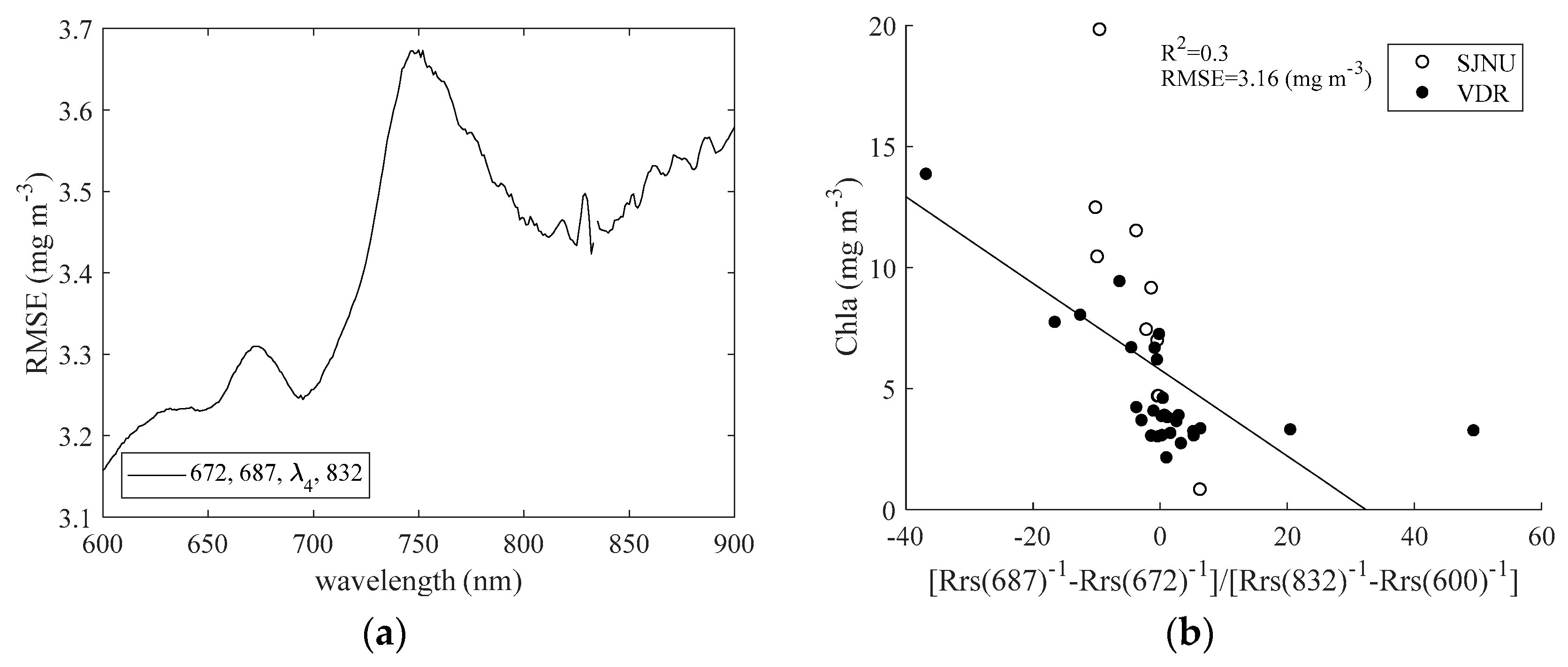
3.2.1. Chla Algorithm

Determining the Chla algorithm’s optimum wavelength position is vital for regional dependency reasons. Previous studies have confirmed changes in R2 and RMSE values by moving the wavelength within a certain range [20,23]. Here, we selected the optimal band with the minimum RMSE as these studies; however, we tried all combinations of 1 nm in the 2-BM.
Figure 4 shows the Chla results from the C1 model in the SJNU and VDR. Figure 4a shows the correlation coefficient matrix [Rrs(λ1)/ Rrs(λ2)] and measured Chla derived every 1 nm in the 400–900-nm range. Rrs values at 687 nm and 672 nm are the highest correlated (R2 = 0.69, RMSE mg m−3), and relatively strong correlation was obtained only in the narrow area noted by the box labeled “A.” Figure 4b shows the optimal [Rrs(687)/Rrs(672)] correlation and measured Chla. Figure 4c,d shows the RMSEs of variation between [Rrs(λ1)/Rrs(672)] or [Rrs(687)/Rrs(λ2)] and measured Chla when λ1 or λ2 is in the 600–900-nm range. Thus, in this model, we obtained a relatively stable RMSE of 1.95 ± 0.05 mg m−3 when λ3 was about 740–900 nm, and the RMSE increases abruptly at wavelengths shorter than 740 nm.
Figure 5 shows the Chla results from the C2 model for in SJNU and VDR. Figure 5a shows RMSE variation between [Rrs−1(687) − Rrs−1(672)] × R(λ3) and measured Chla when λ3 is in the 600–900-nm range. Thus, in this model, we obtained a relatively stable RMSE of 1.95 ± 0.05 mg m−3 when λ3 was about 740–900 nm, and the RMSE increases abruptly at wavelengths shorter than 740 nm. Figure 5b shows the optimal correlation between [Rrs−1(687) − Rrs−1(672)] × R(832) and measured Chla. As a result, we obtained a relatively high correlation (R2 = 0.73, RMSE = 1.96 mg m−3) similar to that in Figure 4b. Moreover, compared the C2 model shows less variation that the C1 model when Chla concentrations are low (<5 mg m−3).
Figure 6 shows the Chla results of the C3 model in SJNU and VDR. Figure 6a shows RMSE variation between [Rrs−1(687) − Rrs−1(672)] × [R(λ4) − R(832)] and measured Chla when λ4 is in the 600–900-nm range. Figure 6b shows the optimal correlation between [Rrs−1(687) − Rrs−1(672)] × [R−1(600) − R−1(832)] and measured Chla. From these results, we determined that the RMSE within this wavelength range was 3.1–3.7 mg m−3, and that estimation accuracy decreased in every band compared to the C2 model shown in Figure 4.
Table 5 shows the optimal Chla model produced using C1, C2 and C3 as summarized above. The Chla estimation error is smaller than the RMSE in the order of C2, C1 and C3.

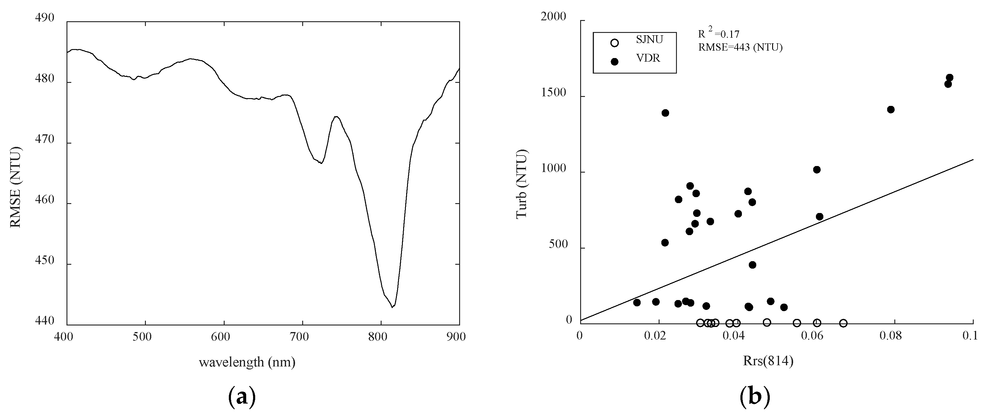
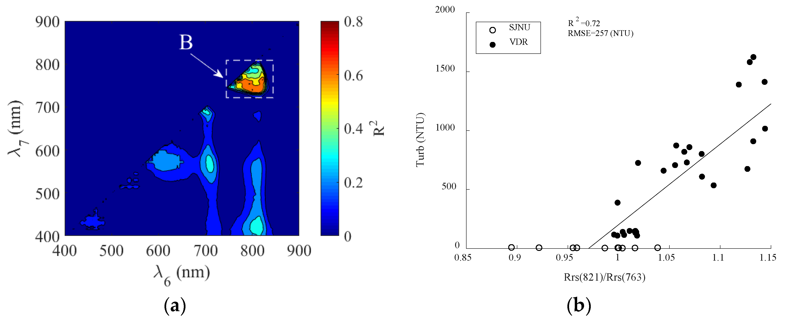
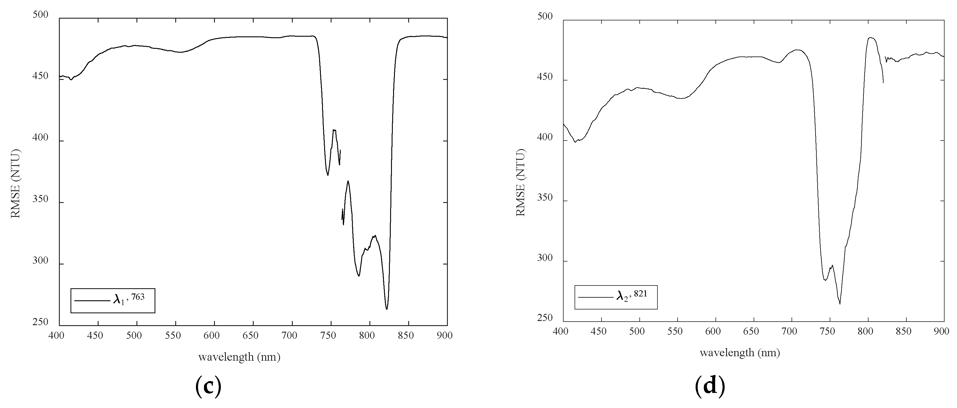
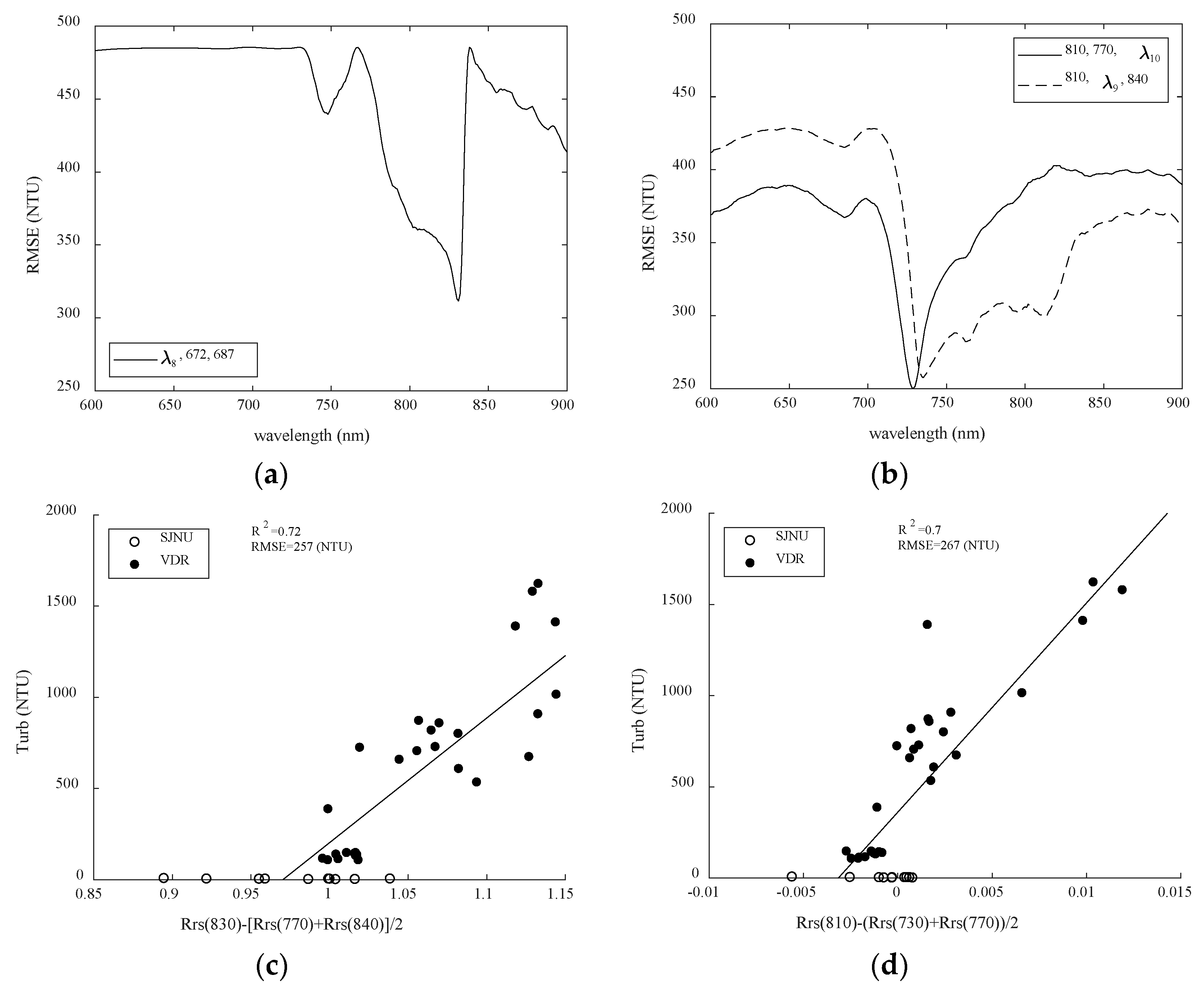
3.2.2. Turbidity Algorithm

As with the Chla algorithm, it is crucial to choose the turbidity algorithm’s optimal wavelength. Here, we performed optimal wavelength selection and evaluation using the same methods as were used with the Chla algorithm.
Figure 7 shows the turbidity results of the one-band model (T1) in SJNU and VDR. Figure 7a shows RMSE variation between Rrs−1(λ5) and measured turbidity when λ5 is in the 400–900-nm range. Figure 7b shows the optimal correlation (R2 = 0.17, RMSE = 443 NTU) between Rrs(814) and measured turbidity. This model’s estimation accuracy of 500 NTU or less was extremely bad.
Figure 8 shows the turbidity results of the two-band model (T2) in SJNU and VDR. Figure 8a shows the correlation coefficient matrix between [Rrs(λ8)/Rrs(λ9)] and measured turbidity. We obtained a relatively strong correlation only in the narrow area indicated by the area labeled “B” in the figure. Figure 8b shows the optimal correlation (R2 = 0.72, RMSE = 257 NTU) between [Rrs(821)/Rrs(763)] and measured turbidity. SJNU data (10 NTU or less) do not appear to be detected in this model. Figure 8c,d shows RMSE variations between [Rrs(λ1)/Rrs(763)] or [Rrs(821)/Rrs(λ9)] and measured turbidity when λ1 or λ2 is in the 400–900-nm range. We obtained a low RMSE value in combination with 763 nm between 740 nm and 820 nm (RMSE = 400 NTU or less). In contrast, the band with low RMSE in combination with 821 nm is between 740 nm and 770 nm (RMSE = 400 NTU or less).
Figure 9 shows the turbidity results of the three-band model (T3) in SJNU and VDR. Figure 9a shows the RMSE variation between Rrs(λ8) − [Rrs(770) + Rrs(840)]/2 and measured turbidity when λ8 is in the 400–900-nm range. We obtained a relatively low RMSE (RMSE = 400 NTU or less) by tuning λ8 between 780 nm and 840 nm. Figure 9b shows the RMSE variation between Rrs(810) − [Rrs−1 (λ9) + Rrs(840)]/2 and measured turbidity when λ9 is the 400–900-nm range and Rrs(810) − [Rrs(770) + Rrs(λ10)]/2 and measured turbidity when λ10 is in the 400–900-nm range. For λ9, we obtained a band with relatively low RMSE (RMSE = 300 NTU or less) between about 730 nm and 770 nm. In contrast, the relatively low RMSE (RMSE = 300 NTU or less) band for λ10 is between about 720 and 740 nm. Figure 9c shows the optimal correlation (R2 = 0.58, RMSE = 316 NTU) between Rrs(830) − [Rrs(770) + Rrs(840)]/2 and measured turbidity. Figure 9d shows the optimal correlation (R2 = 0.70, RMSE = 267 NTU) between Rrs(810) − [Rrs(730) + Rrs(770)] and measured turbidity. Figure 9d seems to be more aggregated data of SJNU compared to Figure 9c.
Table 6 shows the optimal turbidity model using the T1, T2 and T3 models summarized above. Comparing RMSE values shows that the turbidity estimation error is small in the order of T2, T3 and T1.

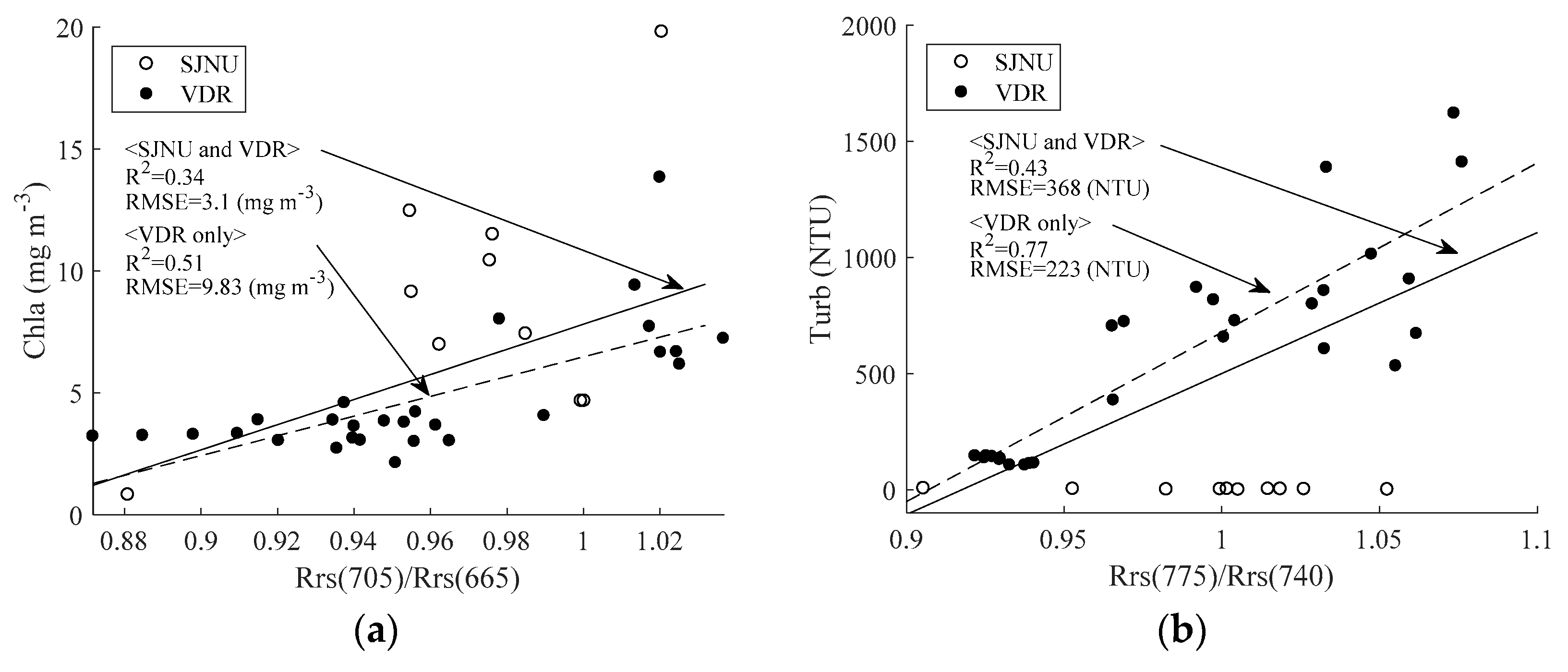
3.3. Algorithm Evaluation Using Simulated Sentinel-2 Data

We evaluated the Chla and turbidity algorithms for satellite observation bands (bands close to the tuned wavelength) using C1, C2, T2 and T3. Figure 10 shows Chla and turbidity results for the 2-BM and 3-BM using the Sentinel-2 MSI band only. Figure 10a shows the correlation between Rrs(705)/Rrs(665) and measured Chla, and Figure 10b shows the correlation between Rrs(775)/Rrs(740) and measured turbidity. Total R2 was low at 0.25 and 0.49 for Chla and turbidity, respectively (RMSE: 3.1 mg m−3 and 347 NTU, respectively); however, R2 slightly improved to 0.51 and 0.77 for Chla and turbidity, respectively (RMSE: 1.5 mg m−3 and 223 NTU, respectively) for the VDR. Figure 10c shows the correlation between [Rrs−1(705) − Rrs−1(665)] × R(842) and measured Chla, and Figure 10d shows the correlation between R(810) − [Rrs(730) + R(770)]/2 and measured turbidity. R2 was not so high at 0.25 and 0.49 for Chla and turbidity, respectively (RMSE = 3.3 mg m−3 and 348 NTU, respectively). However, the correlation improved for the case of VDR data only.
Strong correlations cannot be obtained for all data, as shown in Figure 10a,b; however, the correlation becomes remarkably high only when data are confined to VDR. In such a case, VDR’s spectral reflectance characteristics can be determined mechanically and used as an algorithm with more versatility. We then examined spectral characteristics by separating data from SJNU and VDR. Figure 11a shows the average spectral reflectance characteristics (MSI band only) of all Rrs data in SJNU and VDR. Here, based on the shape of Slope 1 (the slope of Rrs at 705 nm and 740 nm), Slope 2 (the slope of Rrs at 775 nm and 865 nm) and Slope 3 (the slope of Rrs at 775 nm and 865 nm), we focused on the slope of Rrs between the bands. Figure 11b–d shows scatterplots for Slope 1 and Slope 2, Slope 1 and Slope 3 and Slope 2 and Slope 3, respectively. These figures make it clear that data from SJNU and VDR are clearly separated by slope combinations. In particular, in the Slope 1 and Slope 3 scatterplots shown in Figure 11b, SJNU and VDR data were clearly divided between the 1:1 line.

4. Discussion

4.1. Evaluation of Chla Algorithm

As summarized in Table 5, we found the C1 and C2 models to be effective in estimating Chla at the two sites (R2 is about 0.7, RMSE is about 2.0 mg m−3). The four-band model, which is more suitable for detritus-rich water conditions, was found to not be significant under this study’s conditions. We selected 672 nm and 687 nm as the optimal bands for the C1 model, adding 832 nm to these wavelengths for the C2 model. The wavelengths used in the C1 model for water on land were λ1(650–680 nm; red) and λ2(650–720 nm; near infra-red) for a Chla range of about 0–100 mg m−3 [37,38,39,40]. Similarly, for the C2 model, λ1 was 660–670 nm; λ2 was 700–730 nm; and λ3 was 740–760 nm [20,39,40]. The RMSE obtained in these past studies was about 8–10 mg m−3 for a Chla range of 0–100 mg m−3. The Chla range in our study was about one-fifth of those, so it is very harmonious that RMSE was around 2 mg m−3. However, as seen in Figure 4, the wavelength range that can estimate Chla with such RMSE in an algorithm that can be used for both SJNU and VDR is very narrow (about 672 ± 1 nm and 687 ± 1 nm).

4.2. Evaluation of Turbidity Algorithm

The T2 and T3 models were effective (R2 = 0.7, RMSE = 260 NTU), as summarized in Table 6. Furthermore, we selected 821 nm and 763 nm as the optimal bands for T2 and 730 nm, 810 nm and 770 nm as the optimal bands for T3. In previous research, many models used a single band in the red to near-infrared as typified by Chen et al. [24], but when turbidity is extremely high and eutrophic, such as in a watershed, 2-BMs are often used. For example, the combination of 550 nm and 850 nm in France’s Gironde Estuary (TSS: 13–985 g m−3) by Doxaran et al. [27], that of 551 nm and 678 nm (MODIS Bands 12 and 14) in China’s Yellow River (TSS: 2–1897 mg L−1) by Qiu [41] and that of 555 nm and 645 nm in China’s Yangtze River (TSS: 1–300 mg L−1) by Hou et al. [42] were used for 2-BMs. These studies obtained very high correlations with R2 values of 0.8 or more. Because our research sites also have extremely high turbidity and eutrophic water areas, the 2-BM seemed more suitable than a single-band model. Additionally, estimating only turbidity by using a near-infrared wavelength of about 740 nm or more, which is hardly affected by Chla absorption, can be considered appropriate as seen in Figure 1. In contrast, Kutser et al. [29] used bands of 770 nm, 810 nm and 840 nm (T3 model of this study), proposing a new 3-BM targeting the peak near 810 nm in CDOM-rich water areas. This method originally estimates the 810-nm height using the average height of 770 nm and 840 nm as a baseline. The result this time took the average value at 730 nm and 770 nm as the baseline; however, as this idea has just recently been announced, further discussion about which position to use as a baseline will be needed.

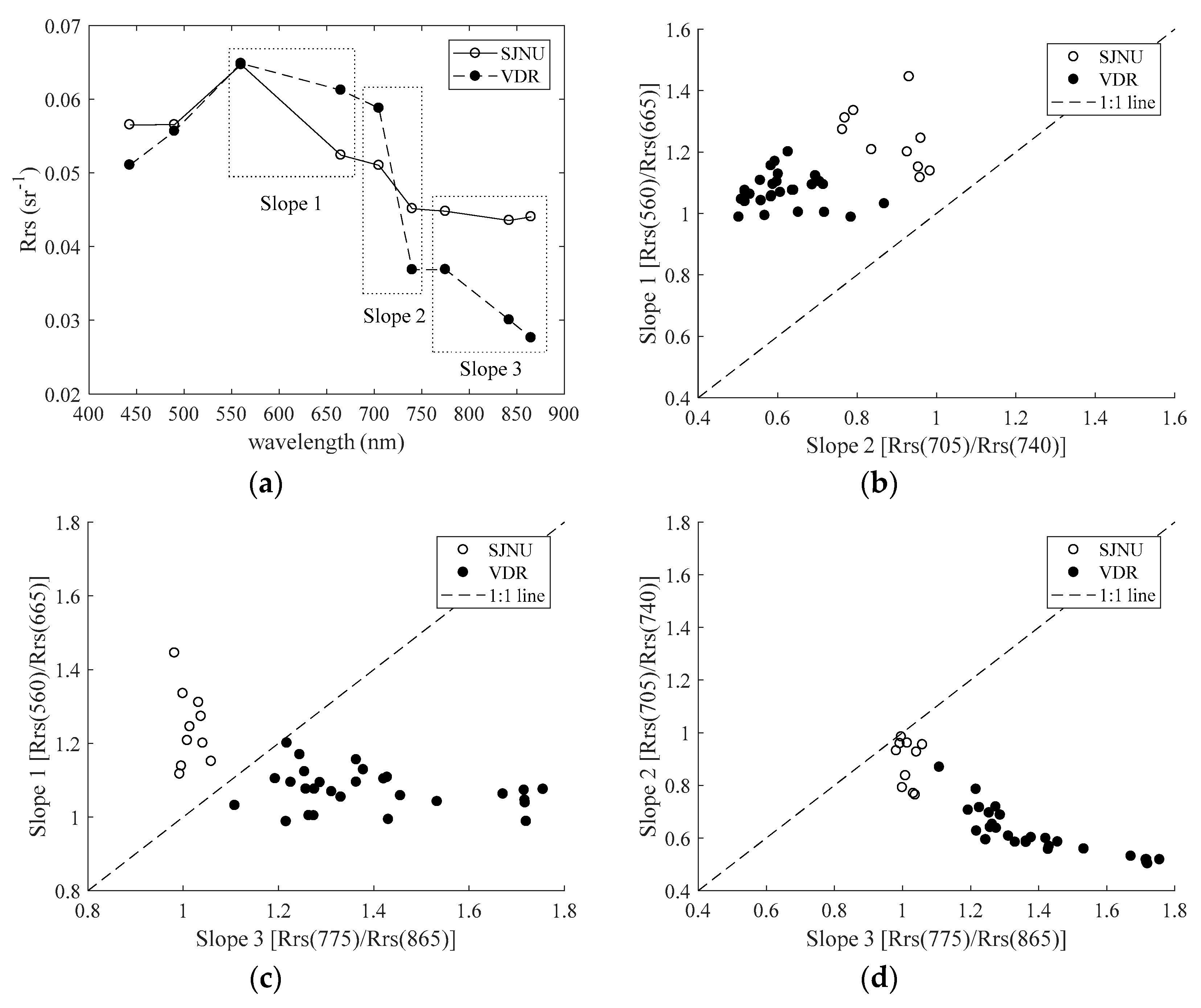
4.3. Feasibilities of Chla and Turbidity Estimation Using the Sentinel-2 MSI Band

In this study, we investigated whether Chla and turbidity can be estimated by MSI’s band, assuming the recently-launched Sentinel-2 MSI, which has high spectral and spatial resolution. As shown in Figure 10, we found no correlation when using all data where both water zones were mixed such that R2 was greater than 0.5 for both Chla and turbidity. However, when only the VDR data were used, we observed a significant correlation (R2 = 0.51, RMSE = 9.8 mg m−3, N = 38) in the 2-BM using 705 nm and 665 nm (MSI Bands 4 and 5). The 2-BM using 775 nm and 740 nm to measure turbidity found a significant correlation (R2 = 0.77, RMSE = 223 NTU, N = 38). SJNU had much lower turbidity measurements than VDR; thus, we found it extremely difficult to find a unified algorithm. Recently, Chen et al. [43] conducted a Chla estimation study targeting MSI bands by measuring the spectral reflectance of Lake Huron (Chla range of 2–52 mg m−3) obtaining 705 nm and 665 nm. In the 2-BM we used, we obtained a correlation of R2 = 0.49 and RMSE = 9.97 mg m−3. In addition, Ha et al. [44] obtained 2-BM R2 values of 0.68 using 560 nm and 665 nm and R2 =0.29 using 705 nm and 665 nm for Vietnam’s Lake Ba Be (Chla range of 1–6 mg m−3). This difference indicates the 705-nm and 665-nm frequencies in the 2-BM as more effective in water areas with advanced eutrophication.
As described above, when the Chla and turbidity algorithms are only effective with VDR data, being able to limit the algorithms that can be used based on spectral characteristics beforehand is convenient. In this case, as shown in Figure 11, it is relatively easy to separate data using the spectral reflectance slope of the 2-BM (specifically the slope of MSI Bands 3 and 4 [Rrs(560) and Rrs(665)] and the slope of MSI Bands 7 and 9 [Rrs(775) and Rrs(865)]. Such spectroscopic separation is often used during remote sensing of red tide. For example, Takahashi et al. [45] proposed a method for separating red tide and non-red tide data by treating normalized water-leaving radiance spectral characteristics as almost equal to Rrs and using the slope of 443 nm and 490 nm and the slope of 490 nm and 555 nm, giving us a method to use. Although different from the subjects in this study, it can be said that the method for separating watershed properties using reflectance gradients can be used as a general and practical method in waters other than SJNU and VDR.

5. Conclusions

We acquired unified Chla and turbidity remote sensing algorithms based on recent Chla and turbidity algorithms using spectral reflectance data acquired by field surveys of SJNU and VDR and evaluating significantly different spectral characteristics. In addition, we also considered Chla and turbidity estimation using Sentinel-2 MSI frequency bands. As a result, we clarified the following items.
  • As a unified Chla model in SJNU and VDR, we obtained strong correlation (R2 = about 0.7, RMSE = 2 mg m−3, N = 38) between Rrs(687)/Rrs(672) (2-BM) or [Rrs−1(687) − Rrs−1(672)] × Rrs(832) (3-BM) and estimated Chla.
  • As a unified turbidity model in SJNU and VDR, we obtained strong correlation (R2 = about 0.7, RMSE = about 260 NTU, N = 38) between Rrs(763)/Rrs(821) (2-BM) or Rrs(810) − [Rrs(730) + Rrs(770)]/2 (3-BM) and estimated turbidity.
  • As a Chla model confined to the MSI frequency band, we obtained strong correlation (R2 = 0.51, RMSE = 9.8 mg m−3, N = 28) between 2-BM using MSI Bands 4 and 5 (Rrs(740) and Rrs(775)) and estimated turbidity.
  • As a turbidity model confined to the MSI frequency band, we obtained strong correlation (R2 = 0.77, RMSE = 0.77, 223 NTU, N = 28) between 2-BM using MSI Bands 6 and 7 (Rrs(740) and Rrs(775)) and estimated turbidity.
  • The method using the slopes of Rrs(560) and Rrs(665) and the slopes of Rrs(775) and Rrs(865) (that is, judgment above and below the 1:1 line) was effective at spectrally separating SJNU data and VDR data.
Validation of these models by applying them to actual MSI data is a crucial step in assessing model viability and accuracy using space-borne satellite images. Additionally, continuous monitoring of water quality changes in the VDR and SJNU through mapping will help dam water management.

Author Contributions

Y.S. was the director of the field survey and this paper. H.Y. and M.A.M.A.E. were the project leaders in the planning and implementation of field campaigns for this research project. Y.Y., S.S., E.A. and J.G.C. performed the field survey execution and analysis, respectively.

Acknowledgments

This study was supported in part by JSPS/NRF (National Research Foundation) Bilateral Joint Research Project, “Future scenarios of Japan and South Africa surface water quality: Under changing climate and land-use” and by JSPS KAKENHI (16H05631 and 17H04625).

Conflicts of Interest

The authors declare no conflict of interest.

Appendix A

Table A1. The summary of dataset used in this study. The Rrs is shown for the Sentinel-2 MSI band only.
ChlaTurbRrs (nm) × 10−5
DateStation(mg m−3)(NTU)443490560705740775842865
15 July 2016SJNU
S-619.7340933859419935472969297429772947
S-36.0364656248694262125957604460126086
S-17.4356695591666058515759586756855887
N-69.1251374866573644004228422540394165
N-17.7654465694694859455675513848144851
Ohashi-Mid6.8344634553530142493938375235183602
12 September 2016SJNU
S-612.2246854801559339993166324932043250
S-311.519472961411,00784406444633162206100
S-110.4055265587651648483731375036413632
Ohashi-Mid0.8155735731579635333290346334433526
28 October 2016VDR
Stn33.238670426959717661634409425836423472
Stn42.970472797918921587735723552547284370
Stn52.585739464050434937462644273023972287
Stn63.787057856143688460673866383632663007
Stn73.165745114551472439362738274023412183
Stn84.081741084240458737992286228018291654
Stn92.972747675123579148112678268920871883
Stn137.2157876898073872587677619838279087561
Stn146.1162178928496962799907845842273746924
Stn156.7141067237517874488876383686958605390
Stn169.6101461367255905884754987522442073831
Stn172.979960076338694160773892400433723183
Stn183.967236104169516547102751292123592194
Stn194.453326122892340230431848195015951487
Stn2013.7138826272903356931501839190015081393
Stn2110.660638364075460338992443252321722072
Stn229.290637534057465938972313245120831969
Stn2311.372353145529615457033920379931332951
27 March 2017VDR
Stn.214.510660596986858877274315404629772639
Stn.223.910670637948971589485083474137093313
Stn.163.711448155263625055533251305723252099
Stn.154.011259806572796671444276401531002826
New-13.813036824145518846542469229515961373
Stn.173.713540784669594053312761256717361462
Stn.83.314644334931602752412668246816821437
Stn.43.314232013543426536871909177012131031
Stn.3′3.2137285429743382278914441335910778
New-23.21467172852510,91696314840446130442594

References

  1. Shiklomanov, I.A. World Water Resources. A New Appraisal and Assessment for the 21st Century; UNESCO: Paris, France, 1998. [Google Scholar]
  2. Simis, S.G.; Ruiz-Verdú, A.; Domínguez-Gómez, J.A.; Peña-Martinez, R.; Peters, S.W.; Gons, H.J. Influence of phytoplankton pigment composition on remote sensing of cyanobacterial biomass. Remote Sens. Environ. 2007, 106, 414–427. [Google Scholar] [CrossRef]
  3. Yamamuro, M.; Koike, I. Diel changes of nitrogen species in surface and overlying water of an estuarine lake in summer: Evidence for benthic-pelagic coupling. Limnol. Oceanogr. 1994, 39, 1726–1733. [Google Scholar] [CrossRef]
  4. Nakamura, Y.; Kerciku, F. Effects of filter-feeding bivalves on the distribution of water quality and nutrient cycling in a eutrophic coastal lagoon. J. Mar. Syst. 2000, 26, 209–221. [Google Scholar] [CrossRef]
  5. Uye, S.; Shimazu, T.; Yamamuro, M.; Ishitobi, Y.; Kamiya, H. Geographical and seasonal variations in mesozooplankton abundance and biomass in relation to environmental parameters in Lake Shinji–Ohashi River–Lake Nakaumi brackish-water system, Japan. J. Mar. Syst. 2000, 26, 193–207. [Google Scholar] [CrossRef]
  6. Kunii, H.; Minamoto, K. Temporal and spatial variation in the macrophyte distribution in coastal lagoon Lake Nakaumi and its neighboring waters. J. Mar. Syst. 2000, 26, 223–231. [Google Scholar] [CrossRef]
  7. Senga, Y.; Seike, Y.; Mochida, K.; Fujinaga, K.; Okumura, M. Nitrous oxide in brackish lakes Shinji and Nakaumi, Japan. Limnology 2001, 2, 129–136. [Google Scholar] [CrossRef]
  8. Yamamuro, M.; Hiratsuka, J.I.; Ishitobi, Y.; Hosokawa, S.; Nakamura, Y. Ecosystem shift resulting from loss of eelgrass and other submerged aquatic vegetation in two estuarine lagoons, Lake Nakaumi and Lake Shinji, Japan. J. Oceanogr. 2006, 62, 551–558. [Google Scholar] [CrossRef]
  9. Sugahara, S.; Kamiya, H.; Suyama, Y.; Senga, Y.; Ayukawa, K.; Okumura, M.; Seike, Y. Influence of hypersaturated dissolved oxygenated water on the elution of hydrogen sulfide and methane from sediment in the dredged area in polyhaline Lake Nakaumi. Landsc. Ecol. Eng. 2015, 11, 269–282. [Google Scholar] [CrossRef]
  10. Taylor, J.C.; van Vuuren, M.J.; Pieterse, A.J.H.; Kriel, J.P. The role of tile Hendrik Verwoerd Dam in the Orange River Project. Civ. Eng. = Siviele Ingenieurswese 1972, 14, 51–61. [Google Scholar]
  11. Braune, E.; Rogers, K.H. Vaal River Catchment: Problems and Research Needs; National Scientific Programmes Unit; CSIR: Pretoria, South Africa, 1987. [Google Scholar]
  12. Grobler, D.C.; Toerien, D.F.; Rossouw, J.N. A review of sediment/water quality interaction with particular reference to the Vaal River system. Water S. Afr. 1987, 13, 15–22. [Google Scholar]
  13. Taylor, J.C.; van Vuuren, M.J.; Pieterse, A.J.H. The application and testing of diatom-based indices in the Vaal and Wilge Rivers, South Africa. Water S. Afr. 2007, 33, 51–59. [Google Scholar] [CrossRef]
  14. Naicker, K.; Cukrowska, E.; McCarthy, T.S. Acid mine drainage arising from gold mining activity in Johannesburg, South Africa and environs. Environ. Pollut. 2003, 122, 29–40. [Google Scholar] [CrossRef]
  15. McCarthy, T.S. The impact of acid mine drainage in South Africa. S. Afr. J. Sci. 2011, 107, 1–7. [Google Scholar] [CrossRef]
  16. Jury, M.R. Economic impacts of climate variability in South Africa and development of resource prediction models. J. Appl. Meteorol. 2002, 41, 46–55. [Google Scholar] [CrossRef]
  17. Matthews, M.W. A current review of empirical procedures of remote sensing in inland and near-coastal transitional waters. Int. J. Remote Sens. 2011, 32, 6855–6899. [Google Scholar] [CrossRef]
  18. Mittenzwey, K.H.; Ullrich, S.; Gitelson, A.A.; Kondratiev, K.Y. Determination of chlorophyll a of inland waters on the basis of spectral reflectance. Limnol. Oceanogr. 1992, 37, 147–149. [Google Scholar] [CrossRef]
  19. Gitelson, A.A. The peak near 700 nm on radiance spectra of algae and water: Relationships of its magnitude and position with chlorophyll concentration. Int. J. Remote Sens. 1992, 13, 3367–3373. [Google Scholar] [CrossRef]
  20. Dall’Olmo, G.; Gitelson, A.A. Effect of bio-optical parameter variability on the remote estimation of chlorophyll-a concentration in turbid productive waters: Experimental results. Appl. Opt. 2005, 44, 412–422. [Google Scholar] [CrossRef] [PubMed]
  21. Yang, W.; Matsushita, B.; Chen, J.; Fukushima, T. Estimating constituent concentrations in case II waters from MERIS satellite data by semi-analytical model optimizing and look-up tables. Remote Sens. Environ. 2011, 115, 1247–1259. [Google Scholar] [CrossRef] [Green Version]
  22. Le, C.; Li, Y.; Zha, Y.; Sun, D.; Huang, C.; Lu, H. A four-band semi-analytical model for estimating chlorophyll a in highly turbid lakes: The case of Taihu Lake, China. Remote Sens. Environ. 2009, 113, 1175–1182. [Google Scholar] [CrossRef]
  23. Le, C.; Hu, C.; Cannizzaro, J.; English, D.; Muller-Karger, F.; Lee, Z. Evaluation of chlorophyll-a remote sensing algorithms for an optically complex estuary. Remote Sens. Environ. 2013, 129, 75–89. [Google Scholar] [CrossRef]
  24. Chen, Z.; Hu, C.; Muller-Karger, F. Monitoring turbidity in Tampa Bay using MODIS/Aqua 250-m imagery. Remote Sens. Environ. 2007, 109, 207–220. [Google Scholar] [CrossRef]
  25. Nechad, B.; Ruddick, K.G.; Park, Y. Calibration and validation of a generic multisensor algorithm for mapping of total suspended matter in turbid waters. Remote Sens. Environ. 2010, 114, 854–866. [Google Scholar] [CrossRef]
  26. Kallio, K.; Kutser, T.; Hannonen, T.; Koponen, S.; Pulliainen, J.; Vepsäläinen, J.; Pyhälahti, T. Retrieval of water quality from airborne imaging spectrometry of various lake types in different seasons. Sci. Total Environ. 2001, 268, 59–77. [Google Scholar] [CrossRef]
  27. Doxaran, D.; Froidefond, J.M.; Castaing, P.; Babin, M. Dynamics of the turbidity maximum zone in a macrotidal estuary (the Gironde, France): Observations from field and MODIS satellite data. Estuar. Coast. Shelf Sci. 2009, 81, 321–332. [Google Scholar] [CrossRef]
  28. Letelier, R.M.; Abbott, M.R. An analysis of chlorophyll fluorescence algorithms for the Moderate Resolution Imaging Spectrometer (MODIS). Remote Sens. Environ. 1996, 58, 215–223. [Google Scholar] [CrossRef]
  29. Kutser, T.; Paavel, B.; Verpoorter, C.; Ligi, M.; Soomets, T.; Toming, K.; Casal, G. Remote sensing of black lakes and using 810 nm reflectance peak for retrieving water quality parameters of optically complex waters. Remote Sens. 2016, 8, 497. [Google Scholar] [CrossRef]
  30. Shen, F.; Zhou, Y.X.; Li, D.J.; Zhu, W.J.; Suhyb Salama, M. Medium resolution imaging spectrometer (MERIS) estimation of chlorophyll-a concentration in the turbid sediment-laden waters of the Changjiang (Yangtze) Estuary. Int. J. Remote Sens. 2010, 31, 4635–4650. [Google Scholar] [CrossRef]
  31. Hu, C.; Chen, Z.; Clayton, T.D.; Swarzenski, P.; Brock, J.C.; Muller–Karger, F.E. Assessment of estuarine water-quality indicators using MODIS medium-resolution bands: Initial results from Tampa Bay, FL. Remote Sens. Environ. 2004, 93, 423–441. [Google Scholar] [CrossRef]
  32. Matthews, M.W.; Bernard, S.; Winter, K. Remote sensing of cyanobacteria-dominant algal blooms and water quality parameters in Zeekoevlei, a small hypertrophic lake, using MERIS. Remote Sens. Environ. 2010, 114, 2070–2087. [Google Scholar] [CrossRef]
  33. Olmanson, L.G.; Brezonik, P.L.; Bauer, M.E. Airborne hyperspectral remote sensing to assess spatial distribution of water quality characteristics in large rivers: The Mississippi River and its tributaries in Minnesota. Remote Sens. Environ. 2013, 130, 254–265. [Google Scholar] [CrossRef]
  34. Oyama, Y.; Matsushita, B.; Fukushima, T.; Matsushige, K.; Imai, A. Application of spectral decomposition algorithm for mapping water quality in a turbid lake (Lake Kasumigaura, Japan) from Landsat TM data. ISPRS J. Photogramm. Remote Sens. 2009, 64, 73–85. [Google Scholar] [CrossRef]
  35. Mobley, C.D. Estimation of the remote-sensing reflectance from above-surface measurements. Appl. Opt. 1999, 38, 7442–7455. [Google Scholar] [CrossRef] [PubMed]
  36. Tan, J.; Cherkauer, K.A.; Chaubey, I. Using hyperspectral data to quantify water-quality parameters in the Wabash River and its tributaries, Indiana. Int. J. Remote Sens. 2015, 36, 5466–5484. [Google Scholar] [CrossRef]
  37. Oki, K.; Yasuoka, Y.; Tamura, Y. Estimation of chlorophyll-a and suspended solids concentration in rich concentration water area with remote sensing technique. J. Remote Sens. Soc. Jpn. 2001, 21, 449–457. [Google Scholar]
  38. Thiemann, S.; Kaufmann, H. Lake water quality monitoring using hyperspectral airborne data—A semiempirical multisensor and multitemporal approach for the Mecklenburg Lake District, Germany. Remote Sens. Environ. 2002, 81, 228–237. [Google Scholar] [CrossRef]
  39. Gitelson, A.A.; Schalles, J.F.; Hladik, C.M. Remote chlorophyll-a retrieval in turbid, productive estuaries: Chesapeake Bay case study. Remote Sens. Environ. 2007, 109, 464–472. [Google Scholar] [CrossRef]
  40. Zimba, P.V.; Gitelson, A. Remote estimation of chlorophyll concentration in hyper-eutrophic aquatic systems: Model tuning and accuracy optimization. Aquaculture 2006, 256, 272–286. [Google Scholar] [CrossRef]
  41. Qiu, Z. A simple optical model to estimate suspended particulate matter in Yellow River Estuary. Opt. Express 2013, 21, 27891–27904. [Google Scholar] [CrossRef] [PubMed]
  42. Hou, X.; Feng, L.; Duan, H.; Chen, X.; Sun, D.; Shi, K. Fifteen-year monitoring of the turbidity dynamics in large lakes and reservoirs in the middle and lower basin of the Yangtze River, China. Remote Sens. Environ. 2017, 190, 107–121. [Google Scholar] [CrossRef]
  43. Chen, J.; Zhu, W.; Tian, Y.Q.; Yu, Q.; Zheng, Y.; Huang, L. Remote estimation of colored dissolved organic matter and chlorophyll-a in Lake Huron using Sentinel-2 measurements. J. Appl. Remote Sens. 2017, 11, 036007. [Google Scholar] [CrossRef]
  44. Ha, N.T.T.; Thao, N.T.P.; Koike, K.; Nhuan, M.T. Selecting the Best Band Ratio to Estimate Chlorophyll-a Concentration in a Tropical Freshwater Lake Using Sentinel 2A Images from a Case Study of Lake Ba Be (Northern Vietnam). ISPRS Int. J. Geo-Inf. 2017, 6, 290. [Google Scholar] [CrossRef]
  45. Takahashi, W.; Kawamura, H.; Omura, T.; Furuya, K. Detecting red tides in the eastern Seto inland sea with satellite ocean color imagery. J. Oceanogr. 2009, 65, 647–656. [Google Scholar] [CrossRef]
Figure 1. Typical absorption from Yang et al. [21] for a*chla, a*tripton, aw, a*cdom. The ad is from Kobayashi and Higa (private note) measured in Tokyo Bay.
Water 10 00618 g001
Figure 2. Study areas and field observation points. (a) Lake Shinji and Lake Nakaumi (SJNU); (b) Vaal Dam Reservoir (VDR).
Water 10 00618 g002
Figure 3. Acquired spectral reflectance (Rrs) characteristics. (a) Lake Shinji and Lake Nakaumi (SJNU); (b) Vaal Dam Reservoir (VDR).
Water 10 00618 g003
Figure 4. Chlorophyll a (Chla) results for the two-band model (C1) in Lake Shinji and Lake Nakaumi (SJNU) and the Vaal Dam Reservoir (VDR). (a) Correlation coefficient matrix between [Rrs(λ1)/Rrs(λ2)] and measured Chla; (b) optimal correlation between [Rrs(687)/Rrs(672)] and measured Chla; (c) root mean square error (RMSE) variation between [Rrs(λ1)/Rrs(672)] and measured Chla when λ1 is in the 600–900-nm range; (d) RMSE variation between [Rrs(687)/Rrs(λ2)] and measured Chla when λ2 is in the 600–900-nm range.
Water 10 00618 g004
Figure 5. Chlorophyll a (Chla) results of the three-band model (C2) in Lake Shinji and Lake Nakaumi (SJNU) and the Vaal Dam Reservoir (VDR). (a) Root mean square error (RMSE) variation between [Rrs−1(687) − Rrs−1(672)] × R(λ3) and measured Chla when λ3 is in the 600–900-nm range; (b) optimal correlation between [Rrs−1(687) − Rrs−1(672)] × R(832) and measured Chla.
Water 10 00618 g005
Figure 6. Chlorophyll a (Chla) results of the four-band model (C3) in Lake Shinji and Lake Nakaumi (SJNU) and the Vaal Dam Reservoir (VDR). (a) Root mean square error (RMSE) variation between [Rrs−1(687) − Rrs−1(672)] × [R(λ4) − R(832)] and measured Chla when λ4 is moved in the 600–900-nm range; (b) optimal correlation between [Rrs−1(687) − Rrs−1(672)] × [R−1(600) − R−1(832)] and measured Chla.
Water 10 00618 g006
Figure 7. Turbidity results of the one-band model (T1) in SJNU and VDR. (a) Root mean square error variation between Rrs−1(λ5) and measured turbidity when λ5 is in the 400–900-nm range; (b) optimal correlation between Rrs(814) and measured turbidity (Turb).
Water 10 00618 g007
Figure 8. Turbidity results of the two-band model (T2) in SJNU and VDR. (a) Correlation coefficient matrix between [Rrs(λ8)/Rrs(λ9)] and measured turbidity; (b) optimal correlation between [Rrs(821)/Rrs(763)] and measured turbidity; (c) root mean square (RMSE) variation between [Rrs(λ1)/Rrs(763)] and measured turbidity when λ1 is in the 400–900-nm range; (d) RMSE variation between [Rrs(821)/Rrs(λ9)] and measured turbidity when λ2 is in the 400–900-nm range.
Water 10 00618 g008aWater 10 00618 g008b
Figure 9. Turbidity results of the three-band model (T3) in SJNU and VDR. (a) Root mean square error (RMSE) variation between Rrs(λ8) − [Rrs(770) + Rrs(840)]/2 and measured turbidity when λ8 is in the 400–900-nm range; (b) RMSE variation between Rrs(810) − [Rrs−1 (λ9) + Rrs(840)]/2 and measured turbidity when λ9 is in the 400–900-nm range and Rrs(810) − [Rrs(770) + Rrs(λ10)]/2 and measured turbidity when λ10 is in the 400–900-nm range; (c) optimal correlation between Rrs(830) − [Rrs(770) + Rrs−1(840)] and measured turbidity; (d) optimal correlation between Rrs(810) − [Rrs(730) + Rrs−1(770)] and measured turbidity.
Water 10 00618 g009
Figure 10. Chlorophyll a (Chla) and turbidity results for the two-band model and three-band model using the Sentinel-2 MSI band only. (a) Correlation between Rrs(705)/Rrs(665) and measured Chla; (b) correlation between Rrs(775)/Rrs(740) and measured turbidity; (c) correlation between [Rrs−1(705) − Rrs−1(665)] × R(842) and measured Chla; (d) correlation between R(810) − [Rrs(730) + R(770)]/2 and measured turbidity.
Water 10 00618 g010aWater 10 00618 g010b
Figure 11. Separation method of the Lake Shinji and Lake Nakaumi (SJNU) and Vaal Dam Reservoir (VDR) types. (a) Average spectral reflectance (Rrs) characteristics (Multispectral Imager band only) of all Rrs data in SJNU and VDR; (b) relationship between Slope 1 (Rrs(560)/Rrs(665)) and Slope 2 (Rrs(705)/Rrs(740)); (c) relationship between Slope 1 (Rrs(560)/Rrs(665)) and Slope 3 (Rrs(775)/Rrs(865)); (d) relationship between Slope 2 (Rrs(705)/Rrs(740)) and Slope 3 (Rrs(775)/Rrs(865)).
Water 10 00618 g011
Table 1. Geographical characteristics of the target area.
AreaCoast LineWater VolumeAverage Depth
Locations(km2)(km)(km3)(m)
Lake Shinji79480.344.5
Lake Nakaumi86640.365.4
Vaal Dam Reservoir3218802.5422.5
Table 2. Summary of standard chlorophyll a (Chla) and turbidity algorithms used in this study. C, chlorophyll; T, turbidity.
Water Quality ParametersModel NameAlgorithm StyleOriginal References
ChlaC1Rrs(λ2)/Rrs(λ1)[18,19]
C2(Rrs(λ1)−1Rrs(λ2)−1) × R(λ3)[20,21]
C3[Rrs(λ1)−1Rrs(λ2)−1]/[Rrs(λ4)−1Rrs(λ3)−1][22,23]
TurbidityT1R(λ5)[24,25]
T2R(λ6)/R(λ7)[26,27]
T3R(λ8) − [R(λ9) + R(λ10)]/2[29]
Representative bands: λ1 = 670, λ2 = 710, λ3 = 740, λ4 = 750, λ5 = 645, λ6 = 850, λ7 = 550, λ8 = 810, λ9 = 770, λ10 = 840.
Table 3. Performance of the Sentinel-2 Multispectral Imager (MSI).
Spatial
SatelliteSensorLaunchResolution (m)Center Wavelength (nm)
Sentinel-2MSIFebruary 201610/20*/60**443**, 490, 560, 665, 705*, 740*, 775*, 842, 865*
Table 4. Chlorophyll-a (Chla) and turbidity range of field data.
LocationsDateChla Turbidity
(mg m−3)(NTU)
MinMaxMinMaxN
L. Shinji and
L. Nakaumi (SJNU)
15 July 20164.719.82.15.96
12 September 20160.812.50.02.34
Vaal Dam Reservoir (VDR)26 October 20162.113.8386167818
27 March 20173.04.610614610
Table 5. The optimal chlorophyll a (Chla) algorithm using the C1, C2 and C3 models.
Model RMSE
NameAlgorithmR2(mg m−3)n
C1Chla = 146.5 × [Rrs(687)/Rrs(672)] − 141.90.692.138
C2Chla = 245.2 × [Rrs(687)−1Rrs(672)−1] × Rrs(832) + 4.2660.732.038
C3Chla = −0.1784 × [Rrs(687)−1Rrs(672)−1]/[Rrs(832)−1Rrs(600)−1] + 5.7770.305.238
Table 6. Optimal turbidity algorithm using the T1, T2 and T3 models.
Model RMSE
nameAlgorithmR2(NTU)n
T1Turb = 10,613 × Rrs(814) + 22.2810.1744338
T2Turb = 6834.7 × Rrs(821)/Rrs(763) − 6632.20.7225738
T3Turb = 114,642 × (Rrs(810) − [Rrs(730) + Rrs(770)]/2) + 361.950.7026738

