Decrease in Snow Cover over the Aysén River Catchment in Patagonia, Chile


1
Laboratory for Analysis of the Biosphere (LAB), University of Chile, Avenida Santa Rosa N° 11315, 8820808 Santiago, Chile
2
University of Aysén, Calle Obispo Vielmo N° 62, 5952039 Coyhaique, Chile
3
Department of Environmental Sciences and Renewable Natural Resources, Faculty of Agricultural Sciences, University of Chile, Avenida Santa Rosa N° 11315, 8820808 Santiago, Chile
*
Author to whom correspondence should be addressed.
Water 2018, 10(5), 619; https://doi.org/10.3390/w10050619
Submission received: 24 February 2018
/
Revised: 2 May 2018
/
Accepted: 3 May 2018
/
Published: 10 May 2018
(This article belongs to the Section Hydrology)
Abstract
:The evidence for global warming can be seen in various forms, such as glacier shrinkage, sea ice retreat, sea level rise and air temperature increases. The magnitude of these changes tends to be critical over pristine and extreme biomes. Chilean Patagonia is one of the most pristine and uninhabited regions in the world, home to some of the most important freshwater reservoirs as well as to evergreen forest, lakes and fiords. Furthermore, this region presents a sparse and weak network of ground stations which must be complemented with satellite information to determine trends on biophysical parameters. The main objective of this work is to present the first assessment on snow cover over the Aysén basin in Patagonia-Chile by using Moderate Resolution Imaging Spectroradiometer (MODIS) data from the period 2000–2016. The MOD10A2 product was processed at 500 × 500 m spatial resolution. The time-series analysis consisted in the application of non-parametric tests such as the Mann–Kendall test and Sen’s slope for annual and seasonal mean of snow covered area (SCA). Data from ground meteorological network and river discharges were also included in this work to show the trends in air temperature, precipitation and stream flow during the last decades. Results indicate that snow cover shows a decreasing non-significant trend in annual mean SCA with a −20.01 km2⋅year−1 slope, and neither seasonal mean shows statistical significance. The comparison with in situ data shows a seasonal decrease in stream flows and precipitation during summer. The hydrological year 2016 was the year with the most negative standardized joint anomalies in the period. However, the lack of in situ snow-monitoring stations in addition to the persistence of cloud cover over the basin can impact trends, creating some uncertainties in the data. Finally, this work provides an initial analysis of the possible impacts of global warming as seen by snow cover in Chilean Patagonia.
1. Introduction
The warming of the climate system and radiative forcing observed since the 1950s have increased the temperature of the atmosphere and oceans, reduced the amount of snow and ice cover, and raised the sea level (3.2 mm⋅year−1) [1]. Snow has decreased in most regions, especially during the spring and summer seasons, due to a positive feedback with the air temperature trend [2]. Over the last three decades in the northern hemisphere, the duration of snow cover has remained stable in North America, while in Eurasia it has decreased (−2.6 ± 5.6 days⋅decade−1) [3]. In the southern hemisphere, however, the general lack of available records makes it impossible to establish a trend [2]. There is evidence, however, of retreating glaciers in the Andes mountain range [4,5,6,7], although no detailed analysis has yet been carried out on the variability in snow cover, which plays a crucial role in water supply for agriculture and hydroelectric energy production, mainly in the southern area of the Andes [8,9].
Monitoring snow and its properties can be very problematic since conventional methods of measuring at high altitude are limited by rugged topography and adverse weather conditions. For this reason, satellite images are useful because they provide information on snow cover in mountainous areas at regular intervals of time [10]. Due to the physical properties of snow, it has a high reflectance in the visible spectrum (0.5–0.7 μm) and high absorption in the shortwave infrared (1.0–3.5 μm), which provide the basis of the Normalized Difference Snow Index (NDSI) for differentiating snow from other types of cover. At the same time, this reflectivity depends on factors such as the snow grain size and shape, the content of liquid water, the depth of the snowpack and the presence of impurities [10,11].
Some of the main snow products that have been derived from remote sensors include snow extent maps and snow albedo, snow grain depth and size, and the snow water equivalent (SWE) [12,13]. At global level, the northern hemisphere has the largest number of available studies and satellite products since it has continuously monitored snow cover since 1960, while in the southern hemisphere, this has only been done on specific regions and in the last decade (excluding Antarctica) [14].
The largest part of the Andes mountain range is in Chile, where it stretches 8000 km and has an average height of 4000 m, nearly all of which is covered in snow during the winter season [15]. Some of the most notable studies on snow levels include those by [16] in the northern zone and their study of how wind impacts snow cover duration patterns in Pascua Lama and the Andes through the use of ablation simulation models. At mid-latitudes, Masiokas et al. [17] analyzed the central region of the Andes and identified a positive correlation with warm phase of the El Niño/Southern Oscillation (ENSO), showing the importance of western air masses in the regulation of mountain snowfall. Between the northern and southern zone, Stehr et al. [18] have studied spatiotemporal dynamics of snow cover over five Andean watersheds, detecting an important decline of snow cover. In the southern zone, [19] have studied the snowpack on the Northern Ice Field using satellite images and meteorological data. However, there is a lack of research on the amount of snowfall in the region of Aysén over the past few decades and how this variation might impact the water scheme of the region’s most important rivers, which have been under consideration for several hydroelectric projects [20]. Likewise, this variability might affect how water is managed regionally for different uses, like drinking water and agriculture, thus leading to unsustainable water-use conditions under future scenarios of lower resource availability. In fact, a decrease in precipitation has been estimated for the coming decades [21,22], which might potentially lead to greater vulnerability and might require water users’ organizations to be created for resource use under a scenario of scarcity. It is for this reason that the main objective of this work is to analyze the spatial and temporal variability of snow cover in the Aysén river basin using satellite images and in situ measurements. The structure of this paper is as follows: Section 2 and Section 3 detail the study area and data used. Section 4 presents the methodology, Section 5 the results and, lastly, Section 6 and Section 7 provide a brief discussion and conclusions.
2. Study Area
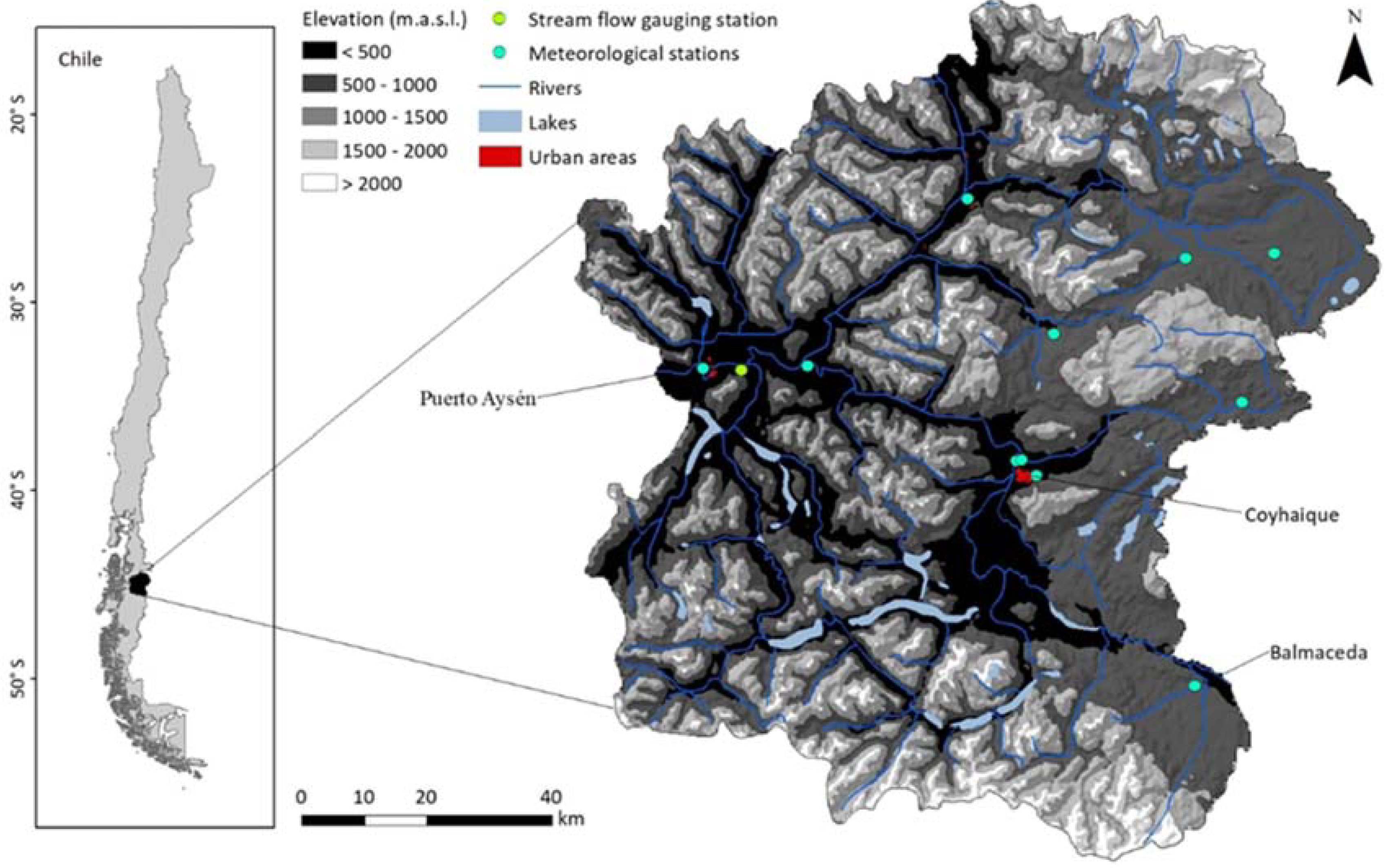
The Aysén river basin (Figure 1) is located in the XI Region of Aysén del General Carlos Ibáñez del Campo between 45° and 46° south latitude. It has a surface area of 11,540 km2, of which 38.3% is covered by native forests, 22.6% by scrub and meadows, and 13.6% by glaciers and permafrost [23].
Its climate is cool oceanic with low temperatures, heavy precipitation and strong winds. However, the different terrain within the basin creates micro-climates: the western sector is influenced by islands and archipelagos and the western slope of the Patagonian Andes, with average annual precipitation between 3000 and 4000 mm and an average annual temperature varying between 8 and 9 °C. The central part of the basin presents a cold steppe climate on the eastern slope of the Patagonian Andes. On the eastern side, rainfall drops as far as 621 mm per year in Balmaceda and down to 1385 mm per year in the city of Coyhaique [24].
The basin has an elevation ranges from the sea level to a high of 2227 m and an average slope of 32%. The western part is where the Andes mountain range intersects and the highest elevations and steepest slopes are found, and where the typical vegetation is temperate, lenga beech forest (Nothofagus pumilio) [25]. The eastern part, on the other hand, has wide valleys and gentle slopes with the Patagonian steppe [26].
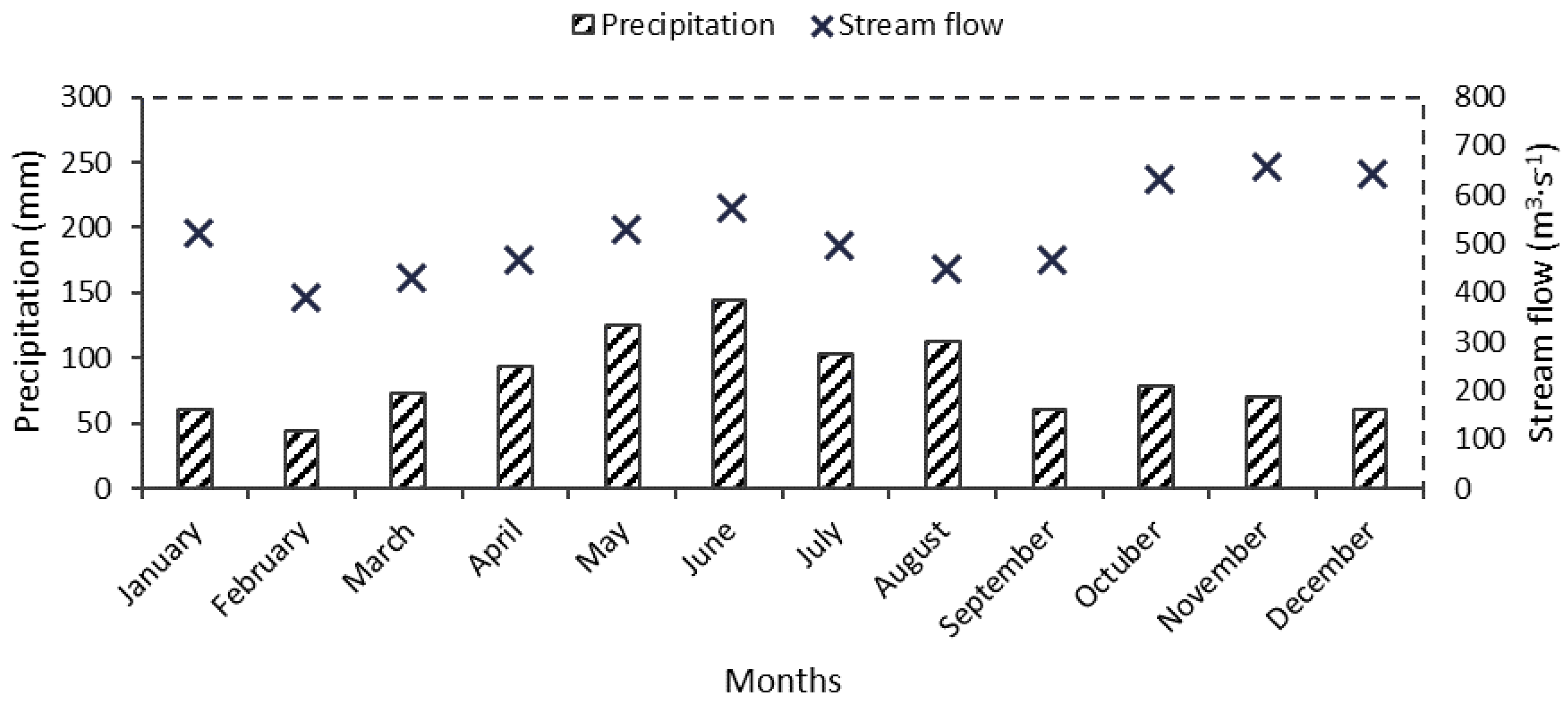
The river basin’s predominant hydrological regime is pluvial-nival (Figure 2), with three sub-regimes: mixed nivo-pluvial in trans-Andean riverbeds, mixed nivo-pluvial and nivo-pluvial regulated by lakes and glaciers. The first sub-regime is characterized by flow coming mainly from melting; the second by the predominance of rainfall as a result of orographic factors; and the third, by the regulation of lakes and glaciers. In this last sub-regime is the Blanco River and 10 other lakes that produce an increase in flows during the dry season, in addition to a several peaks with permafrost [24]. The major tributaries of the main river are the Mañihuales, Simpson, Blanco, Coyhaique and Los Palos rivers, which provide the basin with an average flow of between 250 and 800 m3⋅s−1 [27,28].
3. Data
3.1. Remote Sensing
The Moderate Resolution Imaging Spectroradiometer (MODIS) is a terrestrial remote-sensing system which employs a cross-track mirror and a set of individual sensors to provide images of the Earth surface and clouds in 36 spectral bands in a wavelength range between 0.405 to 14.385 μm. The main purpose of MODIS is to aid in the study of vegetation and its properties, the concentration of aerosols, albedo and surface temperature, as well as snow and ice cover. Snow cover is identified using the Normalized Difference Snow Index (NDSI) [11,29], while snow cover over densely forested areas is identified using thresholds of NDSI along with the Normalized Difference Vegetation Index (NDVI) [30]. MODIS snow cover products are provided daily (MOD10A1) and as 8-day composites (MOD10A2), both at a resolution of 500 m with a sinusoidal map projection. MOD10A2 is a composite of MOD10A1 generated to show maximum snow cover extent [31]. For this study, MOD10A2 (V005) was used to reduce the effects of cloud cover on the study area. The sample period covers the years between 2000 and 2016, with a total of 770 images.
3.2. In Situ Information
In order to compare variations in the snowpack with hydro-meteorological parameters, daily records of average flows (m3⋅s−1), average air temperature (°C) and accumulated precipitation (mm) from stations belonging to the General Directorate of Water (Dirección General de Aguas, DGA) and the Meteorological Directorate of Chile (Dirección Meteorológica de Chile, DMC) were used. Table 1 shows the hydro-meteorological stations and their data availability during the time period.
4. Methods
4.1. Remote-Sensing Processing
To cover the study area, two MOD10A2 (h12v13, h13v13) tiles for the period between 2000 and 2016 were acquired from the National Snow and Ice Data Center (NSIDC) (https://earthdata.nasa.gov/). The images were reprojected into the Universal Transverse Mercator System (UTM) Datum WGS-84 Zone 19S. The original values of the MODIS product were classified into three classes: snow, no-snow (land, continental bodies of water and ocean) and clouds, where the latter corresponded to pixels with no information corresponding to clouds and classes with missing values and errors generated by the sensor (Table 2).
4.2. Snow Covered Area (SCA)
The snow cover corresponding to the reclassified product’s snow class was converted to area by multiplying by a conversion factor of 0.25 km2. This area was presented as snow covered area (SCA).
4.3. Seasonal Trend Analysis
In order to analyze snow cover variation, the average monthly anomalies in SCA were calculated using the method by [32] (Equation (1)):
where is the SCA anomaly, is to the annual/seasonal SCA value, and is the average for the seasonal/annual period for the years in the time series. The trend analysis was performed on the anomaly estimation indicated above, in which the slope among all the ordered pairs on a scatter plot was calculated using Sen’s slope estimator (Equation (2)). In the time series, time will be on the x-axis and SCA on the y-axis. Then, the median of the created data set (mq) was determined and the result represented the non-parametric trend of the sampled time series [33,34],
where mq is the series of slopes among all the combinations of ordered pairs which are natural numbers from 1 to k (Equation (3)):
where n is the total number of ordered pairs. To estimate whether there is a significant trend in the time series, the non-parametric Mann–Kendall test was performed [35,36] since it has been identified as one of the most robust techniques available for estimating trends in environmental variables [37]. Equation (4) gives the statistics on the sign of the trend for the sampled series, where a positive value of t indicates an increasing trend and vice versa:
where signo(x) extracts the sign of the expression entered (Equation (5)).
When the t statistic is calculated with more than 10 data points, it presents a normal distribution, which is what makes it possible to run it through a hypothesis test, for which the z statistic must be calculated as a function of t and its variance (Equation (6)):
To calculate the z-statistic, Equation (7) was used,
The significance level for this work is 0.05, and because it is bilateral, the rejection region of the t statistic will be [Z0.025; Z1–0.025].
4.4. SCA and In Situ Data
The stations whose data availability was equal to or greater than 85% in the period 2000–2016 were used. Hydro-meteorological data were added annually and measurements from the stations were averaged to obtain a representative value at hydrological basin level. As far as precipitation and average air temperature, the annual cumulative and the annual average were used, respectively, as in Equation (8):
where is the annual mean temperature at basin level, is a specific weather station, is the air temperature measurement and is the number of stations in the basin. is the average accumulated precipitation at basin level and is the annual accumulated precipitation measured by one weather station. As far as stream-flow, the annual average of the gauging station at the outlet of the basin was used.
5. Results
5.1. SCA
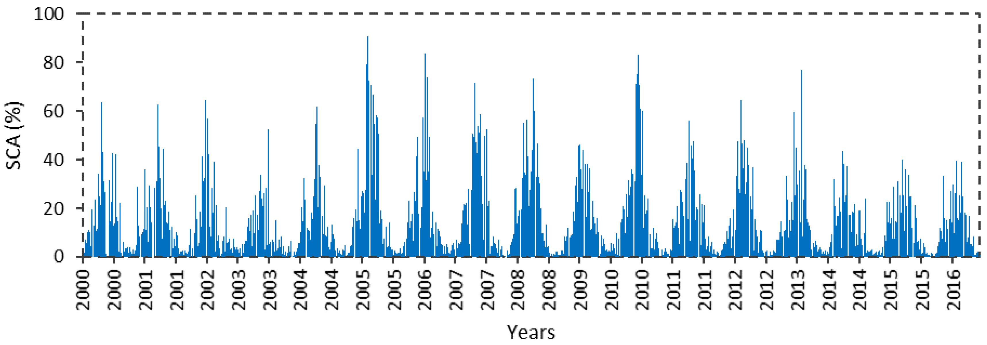
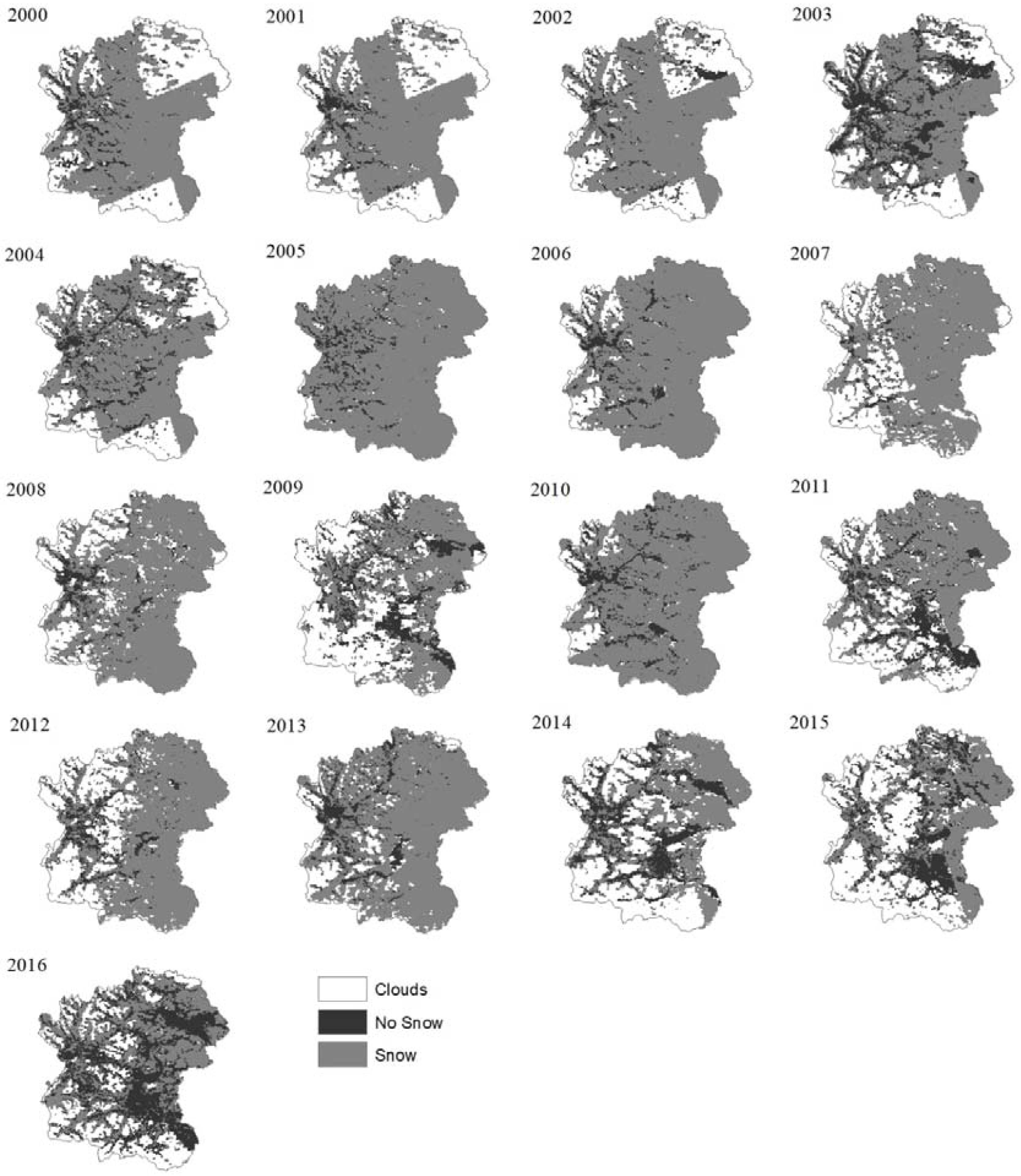
Figure 3 shows the SCA (%) variability for the 2000–2016 period in the Aysén river basin. The greatest SCA accumulation occurs during the winter season and the maximum SCA occurs in the year 2005 when it reaches 90.72%. However, the maximums for the last two years of the period do not exceed 40% of the area of the basin. Figure 4 shows the maximum SCA in each year of the 2000–2016 period.
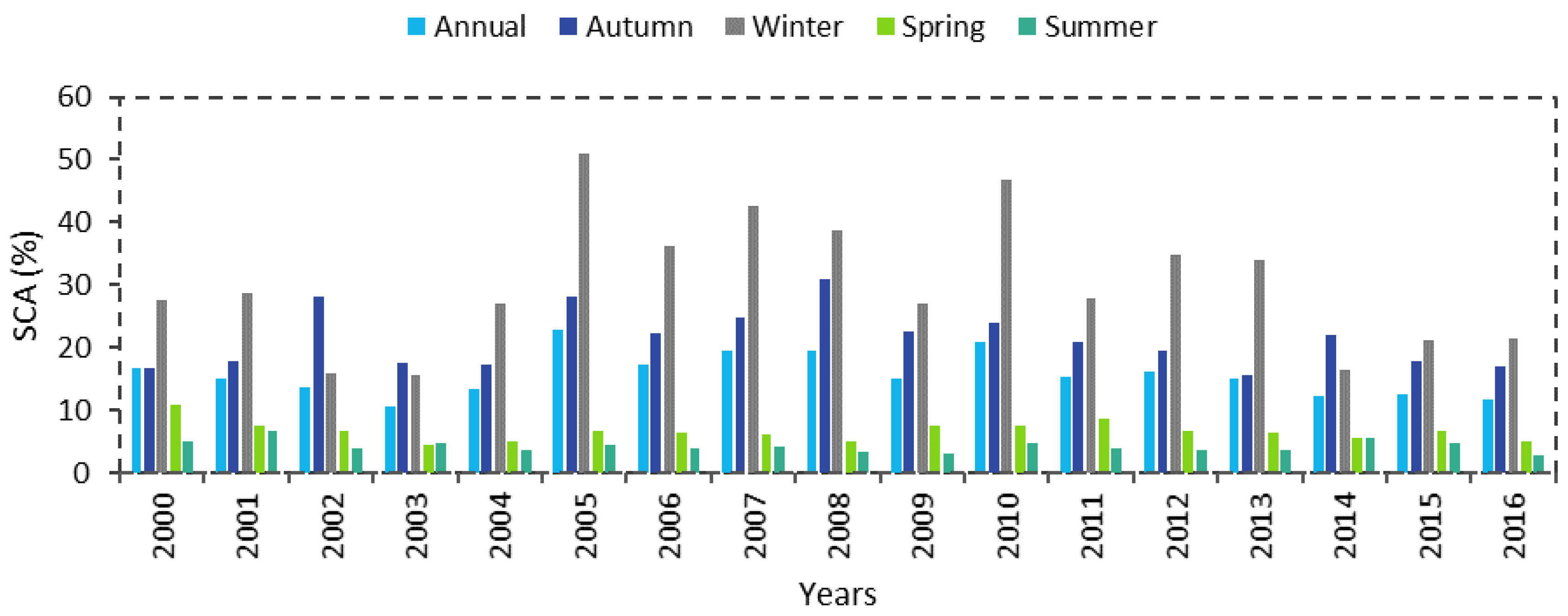
Figure 5 shows the seasonal and annual mean SCA (%) for the 2000–2016 period. The maximum annual mean SCA occur in the years 2005 and 2010, with 22.78% and 20.94% of the basin area, respectively. The greatest accumulation of SCA occurs in the autumn and winter seasons. In autumn, the maximum mean SCA occurs in 2008, while in winter, in the year 2005. In spring, the maximum SCA occurs in the year 2000 and in summer, in the year 2001. The minimum annual mean SCA occur in the years 2003 and 2016.
5.2. Seasonal Trend Analysis
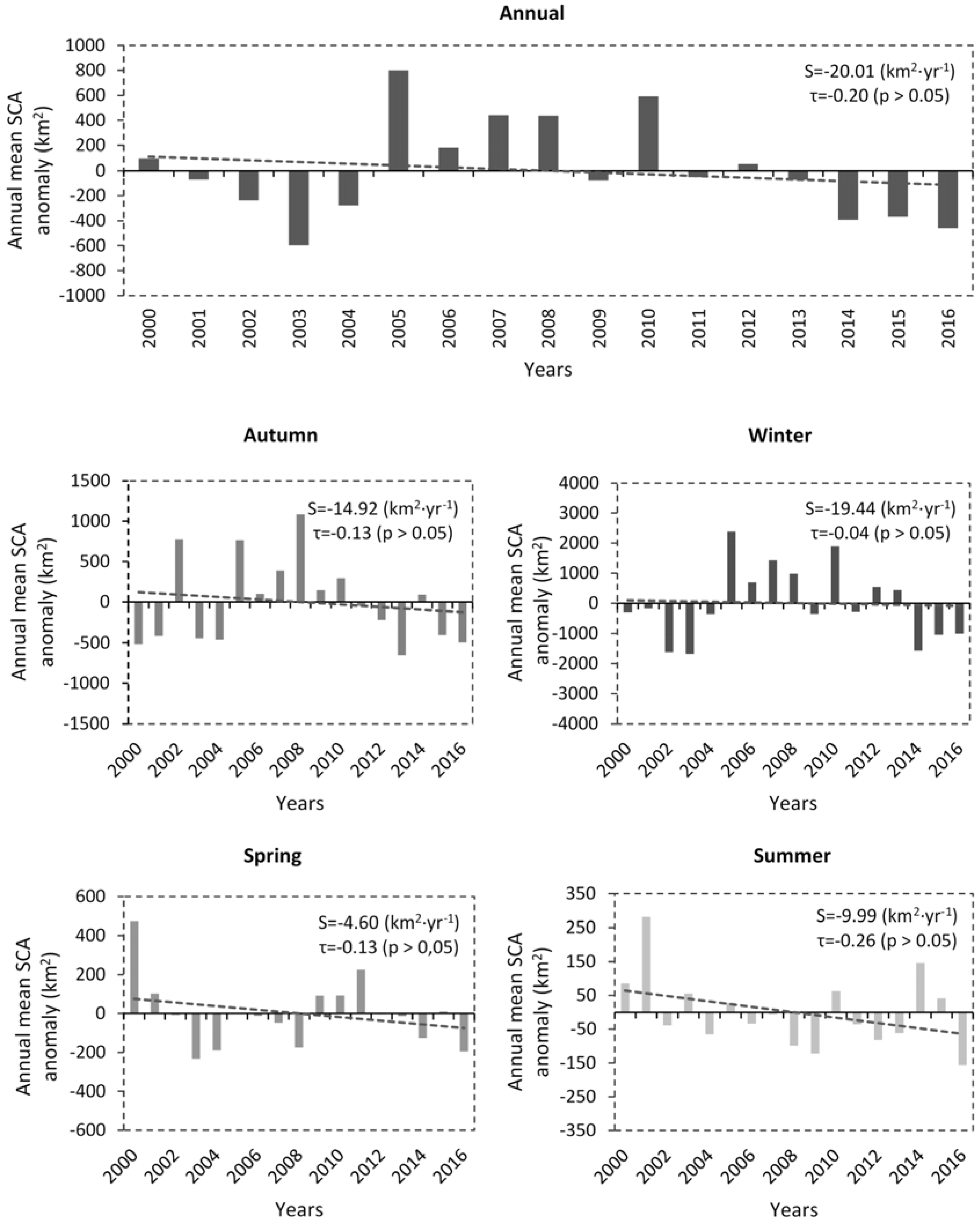
Figure 6 shows the anomalies in the seasonal and annual mean SCA in the 2000–2016 period. Annually, the year 2005 is 801.51 km2 above the average for the period, while the years 2003 and 2016 are 597.20 and 459.49 km2 below the mean for the period, respectively. In addition, during the 2005–2013 period, there are positive or slightly negative anomalies, and then in the following years, there are negative anomalies nearly 400 km2 below the mean for the period. In autumn, the year 2008 presents the maximum positive anomaly, and in 2013 the maximum negative anomaly. In winter, the maximum positive anomaly occurs in 2005 with 2387.11 km2 and in the spring of 2000, with 474.20 km2 above the mean for the 2000–2016 period. In summer, lastly, the maximum anomaly occurs in 2001 with 280.88 km2 above the mean for the time series. Finally, the year 2016 presents the maximum negative anomalies in the spring and summer seasons.
The annual mean SCA shows a non-significant decreasing trend at a rate of −20.01 km2⋅year−1 at 95% confidence. The autumn and winter seasons show decreasing rates of −14.92 and −19.44 km2⋅year−1 with no statistical significance (p > 0.05). In addition, in winter, beginning in 2014, there are negative anomalies of the annual mean SCA of about 1000 km2 below the mean for the 2000–2016 period. Likewise, the spring and summer seasons show non-significant decreasing rates with a slope of −4.60 and −9.99 km2⋅year−1, respectively.
5.3. SCA and In Situ Data
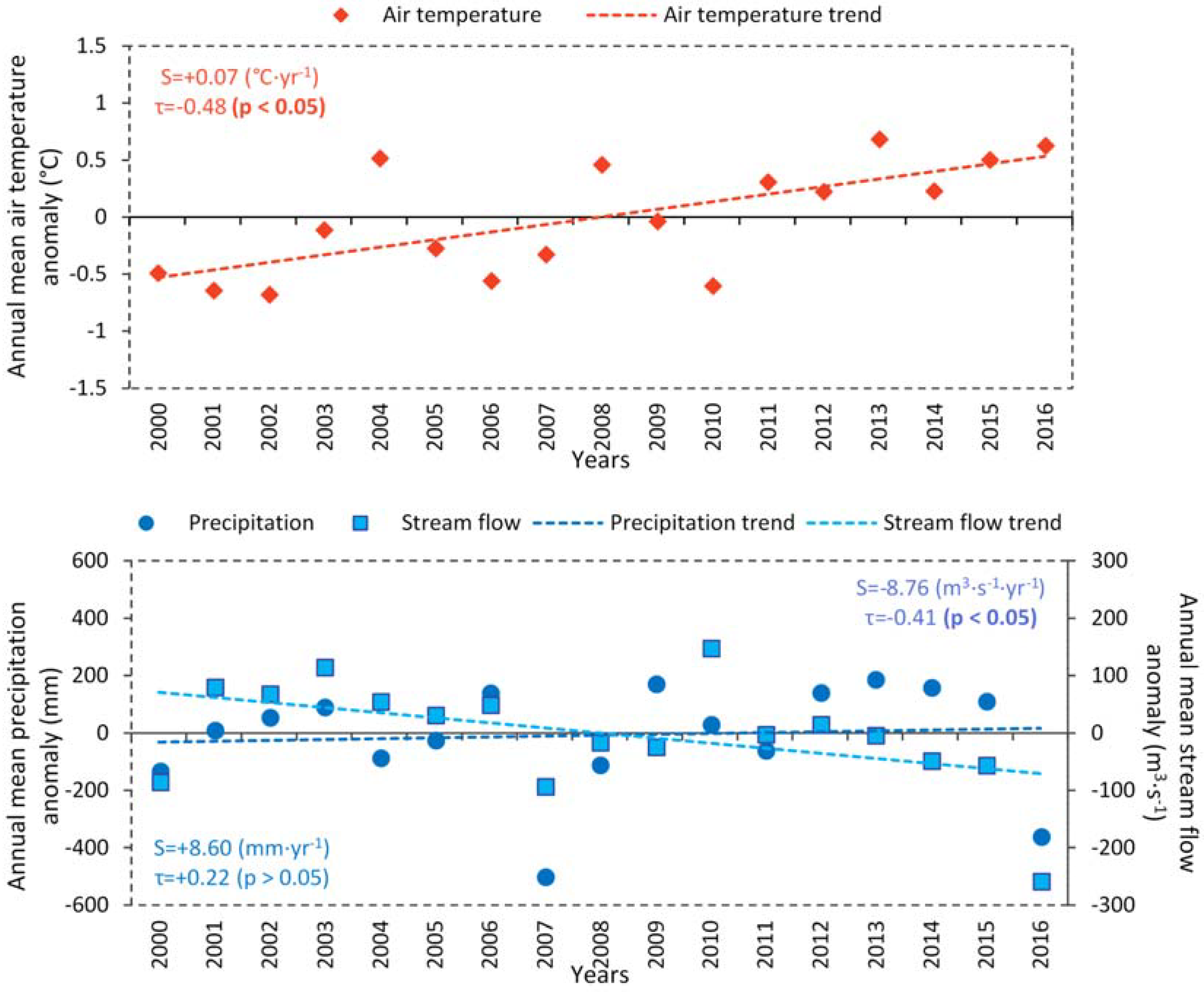
Figure 7 shows the anomalies in the annual mean air temperature, the annual accumulated precipitation and the annual mean stream flows for the Aysén river basin in the period 2000–2016. The air temperature increased significantly, with a trend of +0.07 °C⋅year−1, in which the period 2011–2015 was mainly warm, with 2013 and 2016 as the warmest. On the other hand, the period 2000–2007 was less warm, except for the year 2004, which presents a positive anomaly of 0.53 °C. As far as annual total precipitation, this grew at a non-significant trend +8.60 mm⋅year−1, and in the years 2007 and 2016, it can be seen that there was a significant deficit of over 350 mm compared to the other years in the period 2000–2016. Lastly, annual mean stream flows show a significant decreasing trend with a trend −8.76 m3⋅s−1⋅year−1, as well as a marked decrease in surface runoff in the final five years of the time series. The years 2000, 2007 and 2016 show the most negative anomalies in the period 2000–2016, and in the year 2016 there was a deficit in the annual mean stream flow of −256.81 m3⋅s−1⋅year−1, below the mean for the time series.
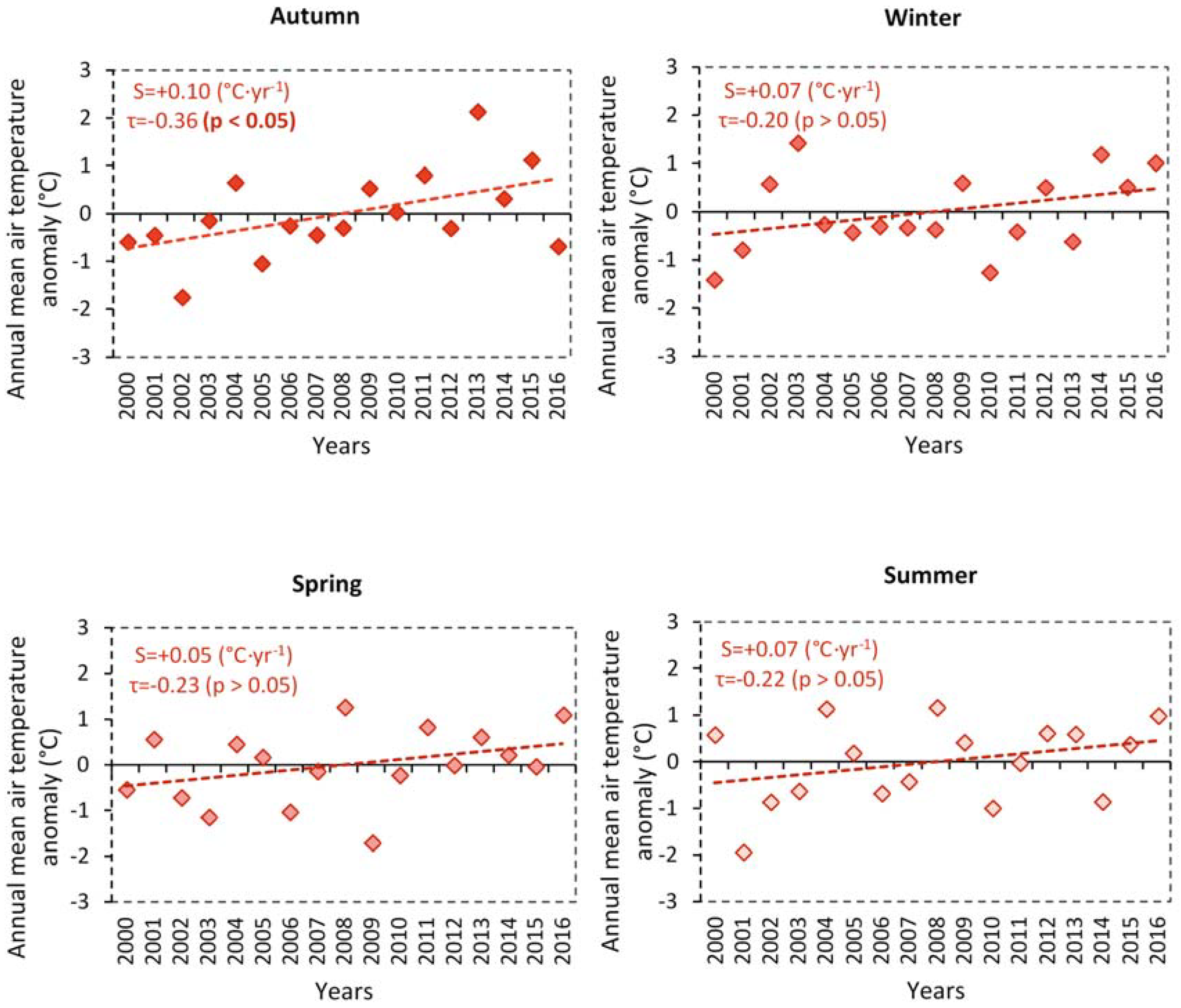
Seasonal trends of mean air temperature anomaly are positive over the study area (Figure 8). For autumn, the time period presents a statistical significance trend (+0.10 °C⋅year−1). It can be seen that positive air temperature anomalies are in relation to the negative SCA anomalies. This effect could be related to the global warming causes, specifically an increase of the 0 °C isotherm, resulting in decreased snow cover in mountainous regions or a reduction in winter snowfall, while also pushing early the thaw in spring [38,39].
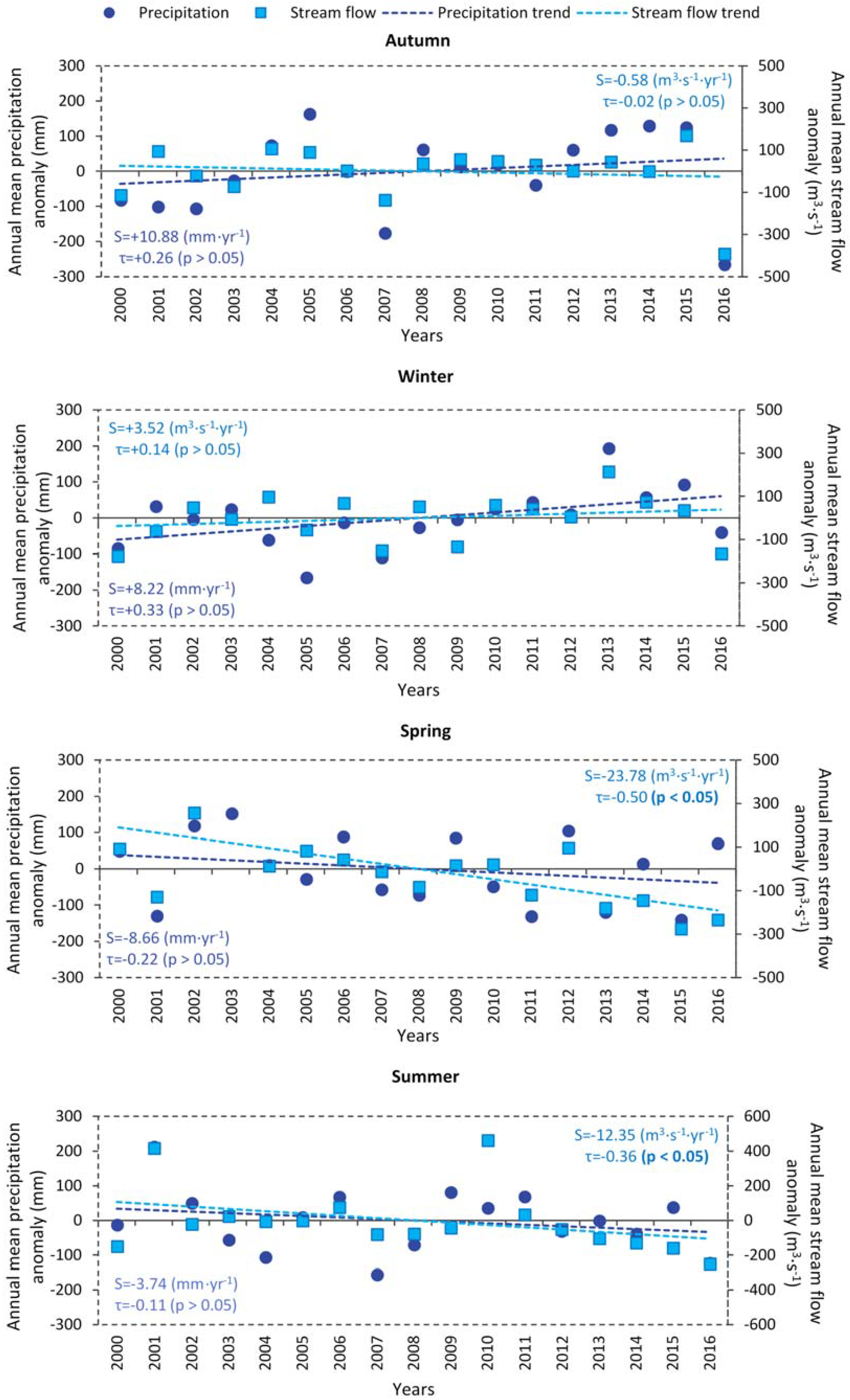
Figure 9 shows the seasonal accumulated precipitation and mean stream flows over the Aysén catchment. Autumn and winter seasons present an increase in precipitation with trends +10.88 mm⋅year−1 and +8.22 mm⋅year−1, respectively. Furthermore, spring and summer show a decrease in precipitation and stream flows, where these latter show a decrease with statistical significance, with slopes of −23.78 and −12.35 m3⋅s−1⋅year−1, respectively. For winter, an increase in stream flows with no statistical significance (p > 0.05) and a slope of +3.52 m3⋅s−1⋅year−1 was estimated.
6. Discussion
The MODIS daily snow product indicates an accuracy of over 90% identifying snow cover under clear sky conditions and its observations are matched to measurements made in situ or taken by other satellites [31,40,41,42,43]. Likewise, in mountain areas with the presence of evergreen forest, the precision of the product decreases up to 75–80% for winter months [44], because thick canopy does not allow the snow to be identified [45]. In this research, a decreasing trend in the annual and seasonal mean of SCA was determined in the Aysén river basin in the period 2000–2016, although with no statistical significance. However, it is necessary to validate these results in future work by incorporating data about snow height and cover measured in situ, which are currently non-existent for the study area. This would improve the estimation of the amount of snow, and not just its surface area, thus improving available estimates.
The last five years in the time period show negative anomalies in the precipitation, streamflow and SCA, with 2016 as the year with the most negative set of anomalies. The variations in snow cover are closely related to the stream flow hydrological response in seasonal cycles. In this sense, generally a positive anomaly of SCA corresponds to a positive anomaly in river discharge in the periods of snow fusion [46]. The SCA shows wide intra- and inter-annual variability, which is consistent with research done in other studies on central Chile and Asia [17,47,48]. In fact, compared to results obtained by [18] in Chile’s Andean basins between latitudes 32.0–39.5° S, there is a decreasing trend in SCA and no significance in the southernmost basins, which is consistent with SCA variability in the Aysén river basin. However, [17] identified a non-significant increasing trend of snowpack over central Chile in the period 1951–2005, which differs from the results of this study due to the fact that it comprises a more extensive data series (54 years) and does not include austral latitudes.
According to [21], a drop in SCA is expected over the Andes mountain range, as well as an increase in the intensity and frequency of extreme climate events related to prolonged droughts and floods. In line with this, central Chile recently experienced the so-called mega-drought in the 2010–2015 period, with a deficit of between 25% and 45% in annual rainfall [49]. During the period from 2000 to 2016, there were five occurrences of El Niño or warm phase of ENSO (2002, 2004–2005, 2006–2007, 2009 and 2015–2016) and three of La Niña (1999–2000, 2007–2008 and 2010–2011) (http://origin.cpc.ncep.noaa.gov/products/analysis_monitoring/ensostuff/ONI_v5.php). In keeping with this, the maximums in annual mean SCA coincide with the periods of La Niña, with the exception of the year 2005. El Niño events are often associated with increases in precipitation, but can also increase the air temperature, which together can have a pronounced altitude effect on the snow cover during spring and fall [50]. In this sense, an increase in air temperature causes 0 °C isotherm to ascend to higher elevations resulting in a larger proportion of precipitation falling as rain as opposed to snow [51,52]. However, due to the short time series of sampled satellite images, it would be necessary to carry out complementary studies to confirm the aforementioned relationship.
The precipitation data used show a limited spatial distribution with respect to the diversity of geographic zones in the study area. In fact, most of the stations are located in sectors near the mouth of the Aysén River, making evident the lack of data in areas of snow accumulation, height, lakeside areas, among others. Likewise, precipitation stations consist of basic rain gauges lacking any adaptations for measuring or determining snowfall. This means that there could be a bias in the data when combining solid and liquid precipitation at the same station. In addition, this study analyzed SCA and not the height or volume of snow, so a greater SCA does not necessarily mean a greater amount of water stored as snow [18].
In terms of management, variability and decreasing precipitation and SCA might potentially require a water-management plan for the basin because a negative trend in snow cover would mean a relatively greater shortage of available water in the basin, thus affecting ways of dealing with a demand that has not been prioritized as of yet in regional management plans and programs. In fact, the region is adapted to a pluvio-nival hydrological regime, and therefore water availability is abundant in the dry season. This means that the greater water demand is offset by an abundance of the resource. However, a decrease in the snowpack might impact the pluvio-nival regime by altering the water supply’s seasonality. In fact, forecast studies show that in the basins of central Chile, significant changes have already been detected in the regimes of the pluvio-nivales rivers, thus leading to a change in its status to pluvial, modifying the time balance between water supply and demand, affecting agricultural and human consumption [53].
7. Conclusions
In this study, an initial approach is presented for evaluating snow cover variability in the Aysén river basin in Chilean Patagonia. Using MODIS satellite images, the region could be monitored over the last 17 years and SCA trends were estimated. SCA values showed a significant decrease between 2010 and 2016 as compared to the historical record, totaling 1050.48 km2 for the entire Aysén river basin. The decreasing trend in snow cover is dropping, −20.01 km2⋅year−1 (p > 0.05), and variables such as temperature were estimated to be positive, +0.07 °C⋅year−1. Seasonal trends for precipitation and stream flows were negative estimated by −8.66 mm⋅year−1 and −23.78 m3⋅s−1⋅year−1 for spring, respectively. Despite the temporal composite method applied to the MODIS imagery, the persistence of cloud cover during a winter might affect the estimates of SCA and, therefore, these retrievals could impact on seasonal SCA trends. Moreover, the data’s scarce spatial representativeness and lack of stations over mountains impact on the validation of the SCA trend and its relation to precipitation, stream flows and air temperature. Nevertheless, this is the first work to contribute to the analysis of snow cover in one of Chilean Patagonia’s most important river basins, where the impact of global warming could have consequences in the water balance and, therefore, impact on the sustainable management of water resources.
Author Contributions
T.P. and C.M. conceived and designed the research. T.P. performed the data processing and analysis. C.M. and R.F. assisted with interpretation and data analysis. All authors contributed to the manuscript write-up and editing.
Acknowledgments
This study was partially financed by the projects “USemilla−Universidad de Aysén” and “Fortalecimiento Institucional en los diversos ámbitos del quehacer universitario, con énfasis en la mejora de su infraestructura, para afrontar los nuevos desafíos de desarrollo institucional 1656 B, Tutorías Universidad de Aysén” −University of Chile. The authors are also grateful for open access to NASA-MODIS products. We extend a special thanks to the anonymous reviewers for their useful comments on this work.
Conflicts of Interest
The authors declare no conflicts of interest.
References
- IPCC (Intergovernmental Panel on Climate Change). Part A: Global and Sectoral Aspects. In Climate Change 2014: Impacts, Adaptation, and Vulnerability; Contribution of Working Group II to the Fifth Assessment Report of the Intergovernmental Panel on Climate Change; Cambridge University Press: Cambridge, UK; New York, NY, USA, 2014. [Google Scholar]
- Bates, B.; Kundzewicz, Z.W.; Wu, S.; Palutikof, J. Climate Change and Water; Technical Paper VI; Intergovernmental Panel on Climate Change (IPCC): Geneva, Switzerland, 2008; pp. 210–225. [Google Scholar]
- Peng, S.; Piao, S.; Ciais, P.; Friedlingstein, P.; Zhou, L.; Wang, T. Change in snow phenology and its potential feedback to temperature in the Northern Hemisphere over the last three decades. Environ. Res. Lett. 2013, 8, 1–10. [Google Scholar] [CrossRef]
- Casassa, G.; Haeberli, W.; Jones, G.; Kaser, G.; Ribstein, P.; Rivera, A.; Schneider, C. Current status of Andean glaciers. Glob. Planet. Chang. 2007, 59, 1–9. [Google Scholar] [CrossRef]
- Durán-Alarcón, C.; Gevaert, C.M.; Mattar, C.; Jiménez-Muñoz, J.C.; Pasapera-Gonzales, J.J.; Sobrino, J.A.; Silvia-Vidal, Y.; Fashe-Raymundo, O.; Chavez-Espiritu, T.W.; Santillan-Portilla, N.; et al. Recent trends on glacier area retreat over the group of Nevados Caullaraju-Pastoruri (Cordillera Blanca, Peru) using Landsat imagery. J. S. Am. Earth Sci. 2015, 59, 19–26. [Google Scholar] [CrossRef]
- Rivera, A.; Acuña, C.; Casassa, G.; Bown, F. Use of remotely sensed and field data to estimate the contribution of Chilean glaciers to eustatic sea-level rise. Ann. Glaciol. 2002, 34, 367–372. [Google Scholar] [CrossRef]
- Rivera, A.; Bown, F. Recent glacier variations on active ice capped volcanoes in the Southern Volcanic Zone (37°–46° S), Chilean Andes. J. S. Am. Earth Sci. 2013, 45, 345–356. [Google Scholar] [CrossRef]
- Key, J.; Goodison, B.; Schöner, W.; Godøy, Ø.; Ondráš, M.; Snorrason, Á. A Global Cryosphere Watch. Arctic 2015, 68, 48–58. [Google Scholar] [CrossRef]
- Stern, N. The economics of climate change. Am. Econ. Rev. 2008, 98, 1–37. [Google Scholar] [CrossRef]
- Dozier, J. Spectral Signature of Alpine Snow Cover from the Landsat Thematic Mapper. Remote Sens. Environ. 1989, 28, 9–22. [Google Scholar] [CrossRef]
- Hall, D.K.; Riggs, G.A.; Salomonson, V.V. Development of methods for mapping global snow cover using moderate resolution imaging spectroradiometer data. Remote Sens. Environ. 1995, 54, 127–140. [Google Scholar] [CrossRef]
- Dietz, A.J.; Kuenzer, C.; Gessner, U.; Dech, S. Remote sensing of snow—A review of available methods. Int. J. Remote Sens. 2012, 33, 4094–4134. [Google Scholar] [CrossRef]
- König, M.; Winther, J.G.; Isaksson, E. Measuring snow and glacier ice properties from satellite. Rev. Geophys. 2001, 39, 1–27. [Google Scholar] [CrossRef]
- Frei, A.; Tedesco, M.; Lee, S.; Foster, J.; Hall, D.K.; Kelly, R.; Robinson, D.A. A review of global satellite-derived snow products. Adv. Space Res. 2012, 50, 1007–1029. [Google Scholar] [CrossRef]
- Barry, R.G. Chapter 5: Regional cases studies. In Mountain Weather and Climate, 3rd ed.; University of Colorado: Boulder, CO, USA, 2008; pp. 421–426. [Google Scholar]
- Gascoin, S.; Lhermitte, S.; Kinnard, C.; Bortels, K.; Liston, G.E. Wind effects on snow cover in Pascua-Lama, Dry Andes of Chile. Adv. Water Resour. 2013, 55, 25–39. [Google Scholar] [CrossRef] [Green Version]
- Masiokas, M.H.; Villalba, R.; Luckman, B.H.; Le Quesne, C.; Aravena, J.C. Snowpack variations in the central Andes of Argentina and Chile, 1951–2005: Large-scale atmospheric influences and implications for water resources in the region. J. Clim. 2006, 19, 6334–6352. [Google Scholar] [CrossRef]
- Stehr, A.; Aguayo, M. Snow cover dynamics in Andean watersheds of Chile (32.0–39.5° S) during the years 2000–2016. Hydrol. Earth Syst. Sci. 2017, 21, 5111–5126. [Google Scholar] [CrossRef]
- Lopez, P.; Sirguey, P.; Arnaud, Y.; Pouyaud, B.; Chevallier, P. Snow cover monitoring in the Northern Patagonia Icefield using MODIS satellite images (2000–2006). Glob. Planet. Chang. 2008, 61, 103–116. [Google Scholar] [CrossRef]
- Silva, E. Patagonia, without Dams! Lessons of a David vs. Goliath campaign. Extr. Ind. Soc. 2016, 3, 947–957. [Google Scholar] [CrossRef]
- Bozkurt, D.; Rojas, M.; Boisier, J.P.; Valdivieso, J. Climate change impacts on hydroclimatic regimes and extremes over Andean basins in central Chile. Hydrol. Earth Syst. Sci. Discuss. 2017. [Google Scholar] [CrossRef]
- Dai, A. Increasing drought under global warming in observations and models. Nat. Clim. Chang. 2013, 3, 52–58. [Google Scholar] [CrossRef]
- Delgado, L.E.; Sepúlveda, M.B.; Marín, V.H. Provision of ecosystem services by the Aysén watershed, Chilean Patagonia, to rural households. Ecosyst. Serv. 2013, 5, 102–109. [Google Scholar] [CrossRef]
- DGA (Dirección General de Aguas). Cuenca del Río Aysén: Diagnóstico y Clasificación de los Cursos y Cuerpos de Agua Según Objetivos de Calidad. 2004. Available online: http://portal.mma.gob.cl/wp-content/uploads/2017/12/Aysen.pdf (accessed on 2 January 2007).
- Torres-Gómez, M.; Delgado, L.E.; Marín, V.H.; Bustamante, R.O. Estructura del paisaje a lo largo de gradientes urbano-rurales en la cuenca del río Aisén (Región de Aisén, Chile). Rev. Chil. Hist. Nat. 2009, 82, 73–82. [Google Scholar] [CrossRef]
- Rondanelli-Reyes, M.J.; Troncoso-Castro, J.M.; León, C.A. Historia vegetal reciente en Patagonia occidental. Análisis palinológico de Laguna Cea (45°40′ S, 72°14′ W), Coyhaique, Chile. Polibotánica 2011, 32, 163–178. [Google Scholar]
- Bizama, G.; Torrejón, F.; Aguayo, M.; Muñoz, M.D.; Echeverría, C.; Urrutia, R. Pérdida y fragmentación del bosque nativo en la cuenca del río Aysén (Patagonia-Chile) durante el siglo XX. Rev. Geogr. Norte Gd. 2011, 49, 125–138. [Google Scholar] [CrossRef]
- Campuzano, F.J.; Leitão, P.C.; Gonçalves, M.I.; Marin, V.; Tironi, H. Hydrodynamical vertical 2D model for the Aysen Fjord. In Perspectives on Integrated Coastal Zone Management in South America; Neves, R., Baretta, J.W., Mateus, M., Eds.; IST Press: Lisboa, Portugal, 2008; pp. 555–566. [Google Scholar]
- Klein, A.G.; Barnett, A.C. Validation of daily MODIS snow cover maps of the Upper Rio Grande River Basin for the 2000–2001 snow year. Remote Sens. Environ. 2003, 86, 162–176. [Google Scholar] [CrossRef]
- Riggs, G.A.; Hall, D.K.; Salomonson, V.V. MODIS Snow Products User Guide to Collection 5. 2006. Available online: https://modis-snow-ice.gsfc.nasa.gov/uploads/sug_c5.pdf (accessed on 2 January 2007).
- Hall, D.K.; Riggs, G.A. Accuracy assessment of the MODIS snow products. Hydrol. Process. 2007, 21, 1534–1547. [Google Scholar] [CrossRef]
- Muster, S.; Langer, M.; Abnizova, A.; Young, K.L.; Boike, J. Spatio-temporal sensitivity of MODIS land surface temperature anomalies indicates high potential for large-scale land cover change detection in Arctic permafrost landscapes. Remote Sens. Environ. 2015, 168, 1–12. [Google Scholar] [CrossRef] [Green Version]
- Sen, P.K. Estimates of the regression coefficient based on Kendall’s tau. J. Am. Stat. Assoc. 1968, 63, 1379–1389. [Google Scholar] [CrossRef]
- Gilbert, R.O. Sen’s Nonparametric Estimator of Slope. In Statistical Methods for Environmental Pollution Monitoring; John Wiley and Sons: Hoboken, NJ, USA, 1987; pp. 217–219. [Google Scholar]
- Mann, H.B. Non-parametric tests against trend. Econometrica 1945, 13, 245–259. [Google Scholar] [CrossRef]
- Kendall, M.G. Rank Correlation Methods; Griffin: Oxford, UK, 1975. [Google Scholar]
- Hess, A.; Iyer, H.; Malm, W. Linear trend analysis: A comparison of methods. Atmos. Environ. 2001, 35, 5211–5222. [Google Scholar] [CrossRef]
- Barnett, T.P.; Adam, J.C.; Lettenmaier, D.P. Potential impacts of a warming climate on water availability in snow-dominated regions. Nature 2005, 438, 303–309. [Google Scholar] [CrossRef] [PubMed]
- López-Moreno, J.I.; García-Ruiz, J.M. Influence of snow accumulation and snowmelt on streamflow in the central Spanish Pyrenees/Influence de l’accumulation et de la fonte de la neige sur les écoulements dans les Pyrénées centrales espagnoles. Hydrol. Sci. J. 2004, 49, 802. [Google Scholar] [CrossRef]
- Zheng, W.; Du, J.; Zhou, X.; Song, M.; Bian, G.; Xie, S.; Feng, X. Vertical distribution of snow cover and its relation to temperature over the Manasi River Basin of Tianshan Mountains, Northwest China. J. Geogr. Sci. 2017, 27, 403–419. [Google Scholar] [CrossRef]
- Zhou, X.; Xie, H.; Hendrickx, M.H.J. Statistical evaluation of remotely sensed snow-cover products with constraints from streamflow and SNOTEL measurements. Remote Sens. Environ. 2005, 94, 214–231. [Google Scholar] [CrossRef]
- Huang, X.; Liang, T.; Zhang, X.; Guo, Z. Validation of MODIS snow cover products using Landsat and ground measurements during the 2001–2005 snow seasons over northern Xinjiang, China. Int. J. Remote Sens. 2011, 32, 133–152. [Google Scholar] [CrossRef]
- Wang, X.; Xie, H.; Liang, T. Evaluation of MODIS snow cover and cloud mask and its application in Northern Xinjiang, China. Remote Sens. Environ. 2008, 112, 1497–1513. [Google Scholar] [CrossRef]
- Simic, A.; Fernandes, R.; Brown, R.; Romanov, P.; Park, W. Validation of VEGETATION, MODIS, and GOES+ SSM/I snow-cover products over Canada based on surface snow depth observations. Hydrol. Process. 2004, 18, 1089–1104. [Google Scholar] [CrossRef]
- Rittger, K.; Painter, T.H.; Dozier, J. Assessment of methods for mapping snow cover from MODIS. Adv. Water Resour. 2013, 51, 367–380. [Google Scholar] [CrossRef]
- Yang, D.; Robinson, D.; Zhao, Y.; Estilow, T.; Ye, B. Streamflow response to seasonal snow cover extent changes in large Siberian watersheds. J. Geophys. Res. Atmos. 2003, 108, 1–21. [Google Scholar] [CrossRef]
- Tang, Z.; Wang, J.; Li, H.; Yan, L. Spatiotemporal changes of snow cover over the Tibetan plateau based on cloud-removed moderate resolution imaging spectroradiometer fractional snow cover product from 2001 to 2011. J. Appl. Remote Sens. 2013, 7, 073582. [Google Scholar] [CrossRef]
- Zhang, G.; Xie, H.; Yao, T.; Liang, T.; Kang, S. Snow cover dynamics of four lake basins over Tibetan Plateau using time series MODIS data (2001–2010). Water Resour. Res. 2012, 48, 1–25. [Google Scholar] [CrossRef]
- Garreaud, R.D.; Alvarez-Garreton, C.; Barichivich, J.; Boisier, J.P.; Duncan, C.; Galleguillos, M.; Zambrano-Bigiarini, M. The 2010–2015 megadrought in central Chile: Impacts on regional hydroclimate and vegetation. Hydrol. Earth Syst. Sci. 2017, 21, 6307–6327. [Google Scholar] [CrossRef]
- Cai, W.; Borlace, S.; Lengaigne, M.; Van Rensch, P.; Collins, M.; Vecchi, G.; England, M.H. Increasing frequency of extreme El Niño events due to greenhouse warming. Nat. Clim. Chang. 2014, 4, 111–116. [Google Scholar] [CrossRef] [Green Version]
- Malmros, J.K.; Mernild, S.H.; Wilson, R.; Tagesson, T.; Fensholt, R. Snow cover and snow albedo changes in the central Andes of Chile and Argentina from daily MODIS observations (2000–2016). Remote Sens. Environ. 2018, 209, 240–252. [Google Scholar] [CrossRef]
- Mernild, S.H.; Liston, G.E.; Kane, D.L.; Knudsen, N.T.; Hasholt, B. Snow, runoff, and mass balance modeling for the entire Mittivakkat Glacier (1998–2006), Ammassalik Island, SE Greenland. Geogr. Tidsskr.-Dan. J. Geogr. 2008, 108, 121–136. [Google Scholar] [CrossRef]
- Vicuña, S.; Meza, F.J. Los nuevos desafíos para la gestión de los recursos hídricos en Chile en el marco del cambio global; Centro de Políticos Publicas de la Pontificia Universidad Católica de Chile: Santiago, Chile, 2012. [Google Scholar]
Figure 1.
Aysén river catchment.

Figure 2.
Intra-annual distributions of mean precipitation and stream flow for the 2000–2016 period.
Figure 2.
Intra-annual distributions of mean precipitation and stream flow for the 2000–2016 period.

Figure 3.
Snow covered area (SCA) variability for the 2000–2016 period.

Figure 4.
Annual maximum SCA for the 2000–2016 period.

Figure 5.
Annual and seasonal mean SCA (%) for the 2000–2016 period.

Figure 6.
Anomalies of annual and seasonal mean SCA for the 2000–2016 period. Mann–Kendall’s trend test “τ” and Sen’s slope estimator “S”.
Figure 6.
Anomalies of annual and seasonal mean SCA for the 2000–2016 period. Mann–Kendall’s trend test “τ” and Sen’s slope estimator “S”.

Figure 7.
Annual mean anomalies for temperature (top), precipitation and stream flow (bottom) for in situ data between 2000 and 2016.
Figure 7.
Annual mean anomalies for temperature (top), precipitation and stream flow (bottom) for in situ data between 2000 and 2016.

Figure 8.
Anomalies of seasonal mean air temperature for the 2000–2016 period.

Figure 9.
Anomalies of seasonal accumulated precipitation and mean stream flow for the period 2000–2016.
Figure 9.
Anomalies of seasonal accumulated precipitation and mean stream flow for the period 2000–2016.


Table 1.
Hydro-meteorological stations located in the Aysén river catchment.
| Station Type * | Station Name | Latitude | Longitude | Altitude (m.a.s.l.) | Data Availability During Period (%) |
|---|---|---|---|---|---|
| M | Villa Mañihuales | 45°10′24″ | 72°08′52″ | 150 | 88.79 |
| M | Estancia Baño Nuevo | 45°16′01″ | 71°31′45″ | 700 | 93.70 |
| M | Ñirehuao | 45°16′14″ | 71°42′33″ | 535 | 74.98 |
| M | Villa Ortega | 45°22′19″ | 71°58′56″ | 550 | 46.46 |
| M | Puerto Aysén | 45°24′02″ | 72°42′00″ | 10 | 71.90 |
| M | El Balseo | 45°24′13″ | 72°29′16″ | 25 | 96.49 |
| M | Rio Aysén en Puerto Aysén | 45°24′21″ | 72°37′23″ | 32 | 86.39 |
| M | Coyhaique Alto | 45°28′49″ | 71°36′16″ | 730 | 77.28 |
| M | Coyhaique CONAF | 45°33′04″ | 72°03′32″ | 340 | 84.38 |
| M | Coyhaique (Escuela Agricola) | 45°34′26″ | 72°01′43″ | 343 | 83.40 |
| M | Puerto Aysén Ad. | 45°23′58″ | 72°40′38″ | 10 | 75.70 |
| M | Teniente Vidal, Coyhaique Ad. | 45°35′38″ | 72°06′31″ | 310 | 100.00 |
| M | Balmaceda Ad. | 45°54′46″ | 71°41′39″ | 517 | 100.00 |
| F | Rio Aysén en Puerto Aysén | 45°24′21″ | 72°37′23″ | 32 | 93.64 |
* Type M is for meteorological weather stations and F for stream-flow gauging station.
Table 2.
MOD10A2 original and reclassified values.
| Original Product | Reclassified Product | ||
|---|---|---|---|
| Value | Description | Value | Description |
| 0 | Missing data | 50 | Clouds |
| 1 | Undetermined | 50 | Clouds |
| 11 | Night | 50 | Clouds |
| 25 | Land | 25 | No snow |
| 37 | Continental water body | 25 | No snow |
| 39 | Ocean | 25 | No snow |
| 50 | Cloud | 50 | Clouds |
| 100 | Ice lake | 200 | Snow |
| 200 | Snow | 200 | Snow |
| 254 | Saturated sensor | 50 | Clouds |
| 255 | Full | 50 | Clouds |
© 2018 by the authors. Licensee MDPI, Basel, Switzerland. This article is an open access article distributed under the terms and conditions of the Creative Commons Attribution (CC BY) license (http://creativecommons.org/licenses/by/4.0/).
Share and Cite
MDPI and ACS Style
Pérez, T.; Mattar, C.; Fuster, R. Decrease in Snow Cover over the Aysén River Catchment in Patagonia, Chile. Water 2018, 10, 619. https://doi.org/10.3390/w10050619
AMA Style
Pérez T, Mattar C, Fuster R. Decrease in Snow Cover over the Aysén River Catchment in Patagonia, Chile. Water. 2018; 10(5):619. https://doi.org/10.3390/w10050619
Chicago/Turabian StylePérez, Tomás, Cristian Mattar, and Rodrigo Fuster. 2018. "Decrease in Snow Cover over the Aysén River Catchment in Patagonia, Chile" Water 10, no. 5: 619. https://doi.org/10.3390/w10050619
Note that from the first issue of 2016, this journal uses article numbers instead of page numbers. See further details here.