Effects of Input Data Content on the Uncertainty of Simulating Water Resources


1
Institute for Landscape Ecology and Resources Management (ILR), Research Centre for BioSystems, Land Use and Nutrition (iFZ), Justus Liebig University Giessen, Heinrich-Buff-Ring 26, 35392 Giessen, Germany
2
Institute of Soil Science and Site Ecology, TU Dresden, Pienner Str. 19, 01737 Tharandt, Germany
3
Centre for International Development and Environmental Research (ZEU), Justus Liebig University Giessen, Senckenbergstraße 3, 35390 Giessen, Germany
*
Author to whom correspondence should be addressed.
Water 2018, 10(5), 621; https://doi.org/10.3390/w10050621
Submission received: 1 March 2018
/
Revised: 4 May 2018
/
Accepted: 8 May 2018
/
Published: 10 May 2018
(This article belongs to the Special Issue Quantifying Uncertainty in Integrated Catchment Studies)
Abstract
:The widely used, partly-deterministic Soil and Water Assessment Tool (SWAT) requires a large amount of spatial input data, such as a digital elevation model (DEM), land use, and soil maps. Modelers make an effort to apply the most specific data possible for the study area to reflect the heterogeneous characteristics of landscapes. Regional data, especially with fine resolution, is often preferred. However, such data is not always available and can be computationally demanding. Despite being coarser, global data are usually free and available to the public. Previous studies revealed the importance for single investigations of different input maps. However, it remains unknown whether higher-resolution data can lead to reliable results. This study investigates how global and regional input datasets affect parameter uncertainty when estimating river discharges. We analyze eight different setups for the SWAT model for a catchment in Luxembourg, combining different land-use, elevation, and soil input data. The Metropolis–Hasting Markov Chain Monte Carlo (MCMC) algorithm is used to infer posterior model parameter uncertainty. We conclude that our higher resolved DEM improves the general model performance in reproducing low flows by 10%. The less detailed soil-map improved the fit of low flows by 25%. In addition, more detailed land-use maps reduce the bias of the model discharge simulations by 50%. Also, despite presenting similar parameter uncertainty (P-factor ranging from 0.34 to 0.41 and R-factor from 0.41 to 0.45) for all setups, the results show a disparate parameter posterior distribution. This indicates that no assessment of all sources of uncertainty simultaneously is compensated by the fitted parameter values. We conclude that our result can give some guidance for future SWAT applications in the selection of the degree of detail for input data.
1. Introduction
Water availability and quality are themes of considerable concern for humanity. Predictions of the consequences of anthropogenic and natural changes in the environment are necessary to understand and support decisions regarding water-resources management, water pollution, and flood control [1,2,3]. Such predictions are made with hydrological models ranging from lumped to fully-distributed setups [4,5,6,7]. However, using a model to mimic the real world has proven to be challenging, due to many possible error sources, such as model structure, input data, forcing data, parameter estimation, and use of goodness-of-fit criteria [8,9,10,11,12,13,14,15,16]. All distributed or semi-distributed hydrological models demand spatial information as input data, such as topography (elevation), LULC (land use/land cover), soils, or (hydro-) geology. These types of data are often available in different resolutions and can be gathered from different sources, with the latter providing some different information, despite having the same resolution [17]. A high-quality reliable input dataset is one of the prerequisites for producing a trustworthy model response by reducing the uncertainty sources [18,19,20].
While there are many hydrological models available for the investigation of data change effects on water quantity [7,21,22,23,24], fewer models are available for studying water quality [25]. This is one reason for the broad application of the Soil and Water Assessment Tool (SWAT) [26], by far the most widely-used hydro-biogeochemical model. In the last few years, the effect of spatial input data on model output has been the focus of hydrological modelling applications [27]. Spatial input data uncertainties are usually associated with source, resample techniques, and resolution.
According to Cotter et al. [28], up to the time of publication no comprehensive study had been done to assess the effect of a digital elevation model (DEM), LULC and soil map resolution on SWAT output error. They resampled these maps to various resolutions, used the maps with the finest resolution to calibrate the model, and transferred the optimum parameters value to the other model setups. The output uncertainty was estimated by the relative error, a measure that compares model output with that originated by the use of the finest resolution. The authors consider that transferring parameter values and not using observed data to calculate relative error would avoid the computation of parameter and observed data uncertainty, respectively. There are some further studies similar to the methodology of Cotter et al. [28] which investigated the sensitivity of streamflow simulation to DEM sources and their and resolutions, LULC resolutions, and different soil information. For example:
DEM sources: Chaubey et al. [29] found an increasing model performance with increasing information of the DEM used when employing SWAT for annual discharge and water-quality simulations. They recommend a minimum DEM data resolution from 100 m to 200 m. Tan et al. [30] evaluated SWAT sensitivity for DEM resolution, DEM resampling techniques, and DEM source. They estimated annual and monthly streamflow without model calibration. The results indicated that SWAT output is more sensitive to DEM resolution than to DEM source and the DEM resampling technique. Lin et al. [31] also investigated impact of DEM resolution on an uncalibrated SWAT. The results indicate no sensitivity to resampling resolution when estimating runoff. Studies on the effect of DEM on SWAT output have also been presented elsewhere [32,33,34].
LULC resolution: Yen et al. [35] investigated the efficiency of parameter transferability used by Cotter el al. [28] and also the sensitivity of SWAT output to different LULC after calibration. The results indicated no sensibility of the model to land-use information provided by LULC. Asante et al. [36] assessed the impact of LULC data resolution on the SWAT model’s predictive uncertainty and showed that low-resolution input data resulted in only slightly smaller model predictive uncertainties. See also [37,38] for similar applications.
Soil information: Chen et al. [39] investigated the effect of soil data sources and resolutions in a mountainous watershed for a non-point source pollution problem. The results indicated a low sensitivity of SWAT to soil data resolution changes and a great impact on model uncertainty depending on the soil data source. Kumar and Merwade [40] investigated the impact of watershed subdivision and soil data resolution, and observed changes in parameter uncertainty using different soil map resolutions. See also [41,42,43] for further studies on soil data uncertainty in SWAT applications.
All these studies demonstrated the importance of spatially distributed input data information to reduce model prediction uncertainty. However, there is not much discussion about the relationship between spatial input data content and uncertainty regarding parameters and input data simultaneously. Surprisingly, the impact of input data uncertainty simultaneously with parameter uncertainty assessment have not yet been described sufficiently in SWAT literature, while it has already shown its importance for rainfall-runoff modelling studies, e.g., [44].
In this study, we investigate the effect of different spatial input data (DEM, LULC and soil maps) on model uncertainty. We use two sources of data for the study:
- (1)
- Global model input datasets, which consider general information and may not represent the heterogeneity of the study area.
- (2)
- Regional model input datasets, with fine resolution of the catchment characteristics, commonly not available for free and computationally demanding.
The aim of this study is to understand how the use of different sources (global and regional) of input datasets may affect the goodness-of-fit of the model and parameter posterior distribution and uncertainty. We hypothesize that finer and regionally-adapted datasets provide higher information content and that SWAT setups based on this type of data have a reduced range of parameter uncertainty and outperform those using global datasets.
2. Materials and Methods
2.1. Study Area
The catchment covers an area of 104 km2, with one-fourth located in the north-west of Luxembourg and three-fourths in the south-east of Belgium (Figure 1). The region is part of the mountainous Ardennes region, with altitudes ranging from 324 to 564 masl. The climate is mild temperate with a total mean annual precipitation of 907 mm from 2006 to 2013. The sparsely-populated area is covered by forests (broad-leaved, coniferous, and mixed), a complex agricultural system and arable lands, pastures, water bodies, and urban areas. The LULC distribution depends on the LULC products being used for this assessment (see also Section 2.3 on LULC data inputs). The prevailing soils developed on schist and sandstone are Cambisol, and Podzols in a few places, showing an overall homogenous distribution of soil types.
2.2. Soil and Water Assessment Tool (SWAT) Model
We used SWAT to simulate hydrological fluxes in the study catchment. SWAT is a semi-distributed, partly physically-based, partly empirical model that requires a diversity of specific information about weather, topography, soil properties, land-management practices, and vegetation [26]. The topographical information is used to delineate the watershed and estimate the surface area and the slope, as well as the stream network and its characteristics, such as length and width. To increase reliability of the latter, SWAT allows the use of a real river network data as burn-in. Additionally, the SWAT user has the option of defining the upstream drainage area, which is required to define the beginning of a stream, providing the opportunity to define how detailed the drainage network is. We set this value to 4.74 km2, as recommend by the ArcSWAT interface. Soil properties and LULC information are used to estimate the land phase of the hydrologic cycle in the model. The land phase controls the amount of water, sediment, and nutrient loadings that flow to the main channel within each sub-basin. A SWAT watershed is partitioned into several sub-basins and then divided into hydrologic response units (HRUs). HRUs are land areas comprised of a unique combination of LULC, land management, soil, and slope. Unlike the sub-basins that are spatially related to one another, there is no information sharing between the HRUs in SWAT, i.e., the different HRUs are modeled separately and are then summed up to determine the total fluxes for the sub-basin in which they are located. We used the ArcSWAT 2012 version, with daily precipitation and minimum and maximum temperatures as forcing data (provided by the Agricultural Technical Services Administration of Luxembourg (ASTA)), and selected the Hargreaves method for estimating daily evapotranspiration rates [45].
2.3. Data Input and Model Setup
The model setup complexity is directly determined by the number of HRUs and sub-basins, which is indirectly defined by the heterogeneity of the input data maps. We analyzed eight different SWAT model setups (Table 1), using input data with various spatial resolution and information content combinations.
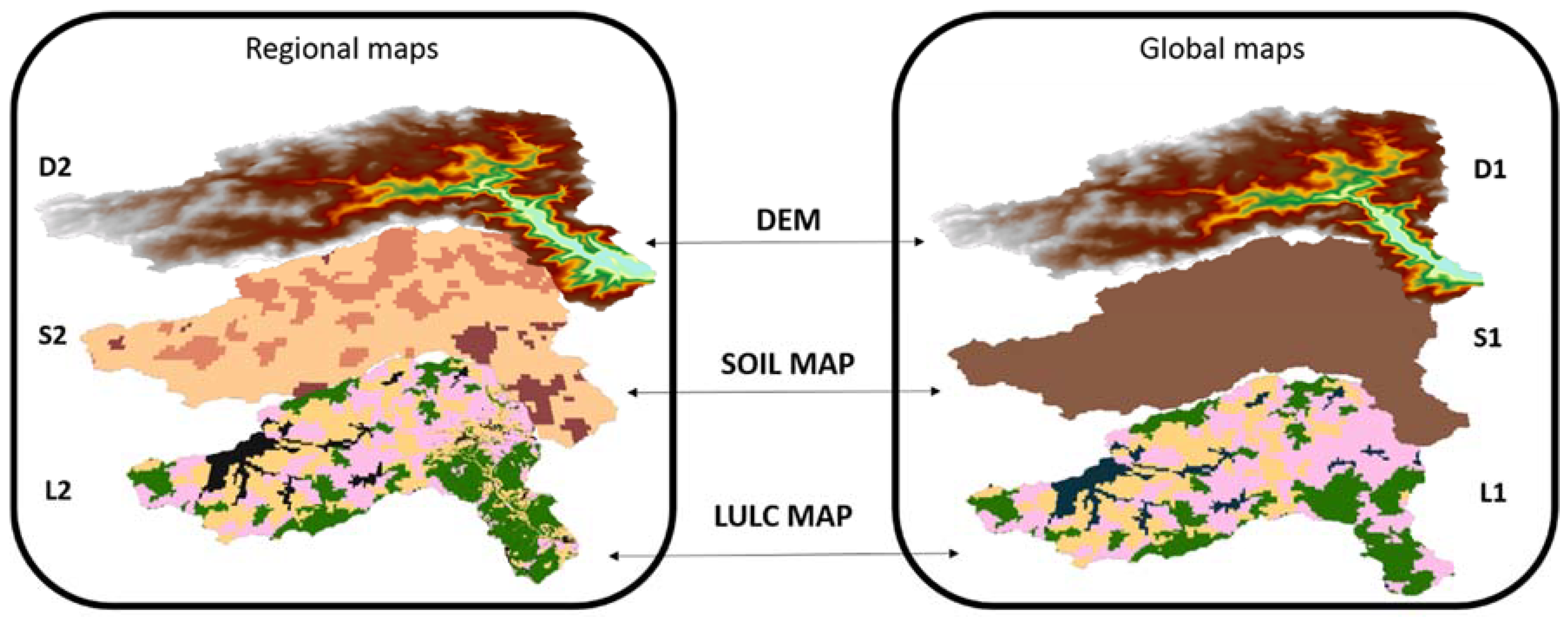
For each data category, we selected a large scale, global map and a more regional data map (Figure 2). The data used in the different setups are described in the following section.
2.3.1. Digital Elevation Model (DEM)
- The pan-European elevation data EU-DEM (D1) is a 3D raster dataset with 30 m resolution and a vertical accuracy of 2.9 m [46,47]. This hybrid product is a weighted averaging of the Shuttle Radar Topography Mission (SRTM) and the Advanced Spaceborne Thermal Emission and Reflection Radiometer (ASTER GDEM).
- The regional DEM (D2) was provided by the Luxembourg Institute of Science and Technology (LIST). The D2 data has a spatial resolution of 5 m.
To match the spatial resolution of D1, the D2 DEM was resampled to 30 m using bilinear interpolation. This reinforces our goal of focusing on different information contents rather than the effect of spatial resolution, which has been investigated elsewhere [48]. The use of different DEM sources affects the watershed delineation, resulting in different terrain characteristics and physical structures of the stream network (Table 1), which is expected to influence model performance [32,40,49]. Before discretizing the watershed into eight sub-basins, we used the same upstream drainage threshold for the area required to form the beginning of a stream (4.74 km2), because Wu et al. [50] reported that different thresholds may affect the streamflow. Additionally, the watershed was classified into three land-slope classes: <7%, 7–15% and >15% that are considered moderate, medium and steep slopes, respectively, according to German guidance for soil surveying and mapping [51].
2.3.2. Land Use/Land Cover (LULC)
- The pan-European CORINE Land Cover 2006 (L1) is a compilation of national LULC datasets. Its production was based on agreed methodology and carried out by the European Environment Agency (EEA) under the framework of the Copernicus program [52]. L1 has a 100 m spatial resolution and represents the LULC status close to the year 2006 with an accuracy above 85%.
- The regional LULC map (L2) titled Occupation Biophysique du Sol (2007) was also provided by the LIST.
We used the same LULC categories for both maps (global and regional), which are forest (including broad-leaved, coniferous, and mixed), pasture, agriculture, water, and urban area. Comparing the categories’ distribution for both maps, the global map has a substantially larger area of agricultural land than the regional map (43.4% vs. 34.5%) and in turn, smaller shares of pasture (24.9% vs. 32.0%), forest (24.0% vs. 25.2%), surface water bodies (0% vs. 0.01%), and urban areas (7.7% vs. 8.3%). We used the same crop rotation calendar for all setups, taking yearly turns of winter wheat and corn that include fertilization, ploughing, planting, and harvest. The fertilization process comprises yearly amounts of phosphorus for winter wheat and corn (60 kg ha−1 and 48 kg ha−1, respectively) as well as nitrogen (174 kg ha−1 and 140 kg ha−1, respectively).
2.3.3. Soils
- The Harmonized World Soil Database (HWSD, version 1.21) (S1) is a 1 km spatial resolution global soil map produced jointly by the International Institute for Applied Systems Analysis IIASA and the Food and Agriculture Organization of the United Nations (FAO) [53]. The database includes commonly used soil parameters and texture classes. S1 presents one soil class for the Wiltz watershed having two layers, one 0.3 m deep and the other 1 m deep.
- SoilGrids (S2) is a 250 m spatial resolution global soil database developed jointly by International Soil Reference and Information Centre (ISRIC—World Soil Information) and other collaborators [54]. S2 has six soil layers with depths of 0.05 m, 0.15 m, 0.30 m, 0.60 m, 1.00 m, and 2.00 m. It provides standard soil properties (soil texture, bulk density, soil organic carbon content, etc.) per each grid cell and layer. To adjust the database to the necessity of SWAT input format, we categorized the cell values according to the soil texture, separating them into three classes: (i) loamy sands and silty-loamy sands with a high percentage of sand and a low percentage of clay (≤17%); (ii) silty loams with a high percentage of silt ≥50%; (iii) and sandy loams and slightly clayey loams with clay >7% and silt <50%.
After defining soil texture values for both maps (global and regional), we calculated SWAT soil physical parameters using the pedotransfer function (PTF) developed by Saxton and Rawls [55]. The soil albedo was calculated using the Baumer equation that is based on the percentage of organic material content [56].
The number of HRUs created by the SWAT model setup is based on the quantity and spatial distribution of LULC, soil, and slope classes. Interpreting the number of HRUs as the setup complexity, the simplest setups use S1 (D2S1L1 and D1S1L1) and have 89 and 90 HRUs, respectively, while the most complex setups use S2 and have 200 HRUs and 199 HRUs (D2S2L2 and D1S2L2, respectively) (Table 1). When defining the HRUs, SWAT allows the use of a threshold for soil, LULC, and slope to reduce the complexity of the model setup. However, we are not using any threshold, because we want to avoid loss of both information and diversity representation.
2.4. Calibration, Parameters, and Uncertainty Analysis
We considered daily discharge measured at the main outlet of the catchment for model validation, (49°58′04′′ E, 5°53′23′′ N). Because of the lack of measure discharge as point source for each sub-basin coming from effluents to the channel network, we considered 19% of the capacity of each wastewater treatment plant (WWTP) in the area. The data for the WWTPs were gathered from the Luxembourgish Intercommunal Syndicate of Wastewater Remediation of the Northern (SIDEN).
We ran SWAT for the period of 2006 to 2013, duplicating the first two years (2006–2007) as warm-up period and using the last two years (2012–2013) to validate the results.
For the model calibration and parameter uncertainty analysis, we used the widely accepted Metropolis–Hasting Markov Chain Monte Carlo (MCMC) algorithm [57] as implemented in the SPOTPY Python package [58]. The SPOTPY package is an open-source tool that simplifies the link between models and Bayesian, optimization, and sensitivity analysis methods. Once the user connects the model to SPOTPY, testing the effects of different analysis strategies and analyzing the model performance is straightforward. The package allows the choice among 12 algorithms for calibration, 9 pre-built parameter distribution functions, 16 objective functions, and 21 likelihood functions.
SWAT was calibrated for daily discharge from the main watershed outlet point. The selection of the six model parameters to be calibrated is based on expert-knowledge. We excluded several parameters that are widely used in SWAT calibration [59,60,61], but are closely related to one of the inputs we were concerned with analyzing (DEM, soil, and LULC maps). Examples include the curve number, saturated hydraulic conductivity, and available water capacity of the soil layer. We focused our analysis on six parameters related to snow, groundwater, and main channel processes, which are described in Table 2, including their respective prior uncertainty range.
We assumed a non-informative uniform prior distribution for the parameters, which were sampled 200,000 times in five parallel chains, maximizing a logarithmic likelihood function:
where is observed data, y is simulated data, θ is parameter set, σ is the measurement error of observed data, t is the time step, and n is total number of observations [62].
We used the multivariate approach proposed by Brooks and Gelman [63] to monitor the chain’s degree of convergence (). Convergence is achieved when the parameter variance within a chain and the variance between chains become indistinguishable, generating a value close to one. Large values indicate a notable difference between chains. The posterior distribution was defined taking in consideration a warm-up period of one-fourth of the simulation length and the convergence criteria < 1.2 in order to generate the posterior parameter distribution.
We assessed model performance calculating the Nash–Sutcliffe Efficiency (NSE), the logarithmic NSE (log NSE), and the percent bias (PBIAS) for the posterior distribution. NSE is defined as the magnitude of residual variance normalized by the observed data variance [64]. Negative values indicate that the mean observed data is a better predictor than the model simulation, whereas values between 0.5 and 1 are considered a good model fit [65]. The squared residuals of the NSE calculation overemphasize high values [10,66]; therefore, we also considered the logarithmic NSE [67], which is more sensitive to low flows than NSE [66,68]. This metric can be interpreted similarly to NSE, where a good performance is achieved when the log NSE is greater than 0.5. PBIAS is determined by the difference between observed and simulated data, normalized by the observed discharge [69]. Model accuracy is characterized by low values, i.e., the metric has zero set as the optimum value, and values between −3 and 3 are considered a good performance. Moreover, a positive PBIAS value represents a model toward underestimation and a negative value a model toward overestimation [69].
Part of model uncertainty was estimated using the measured P- and R-factors [70]. The P-factor is the percentage of data bracket by the 95% prediction uncertainty (95PPU) which is calculated at the 2.5 and 97.5 percentiles of the simulated data. The R-factor is the ratio of the average distance between the upper and lower 95PPU and the standard deviation of the measured data. Ideally, the P-factor tends to 1 and the R-factor is close to 0.
3. Results and Discussion
3.1. Posterior Model Performance
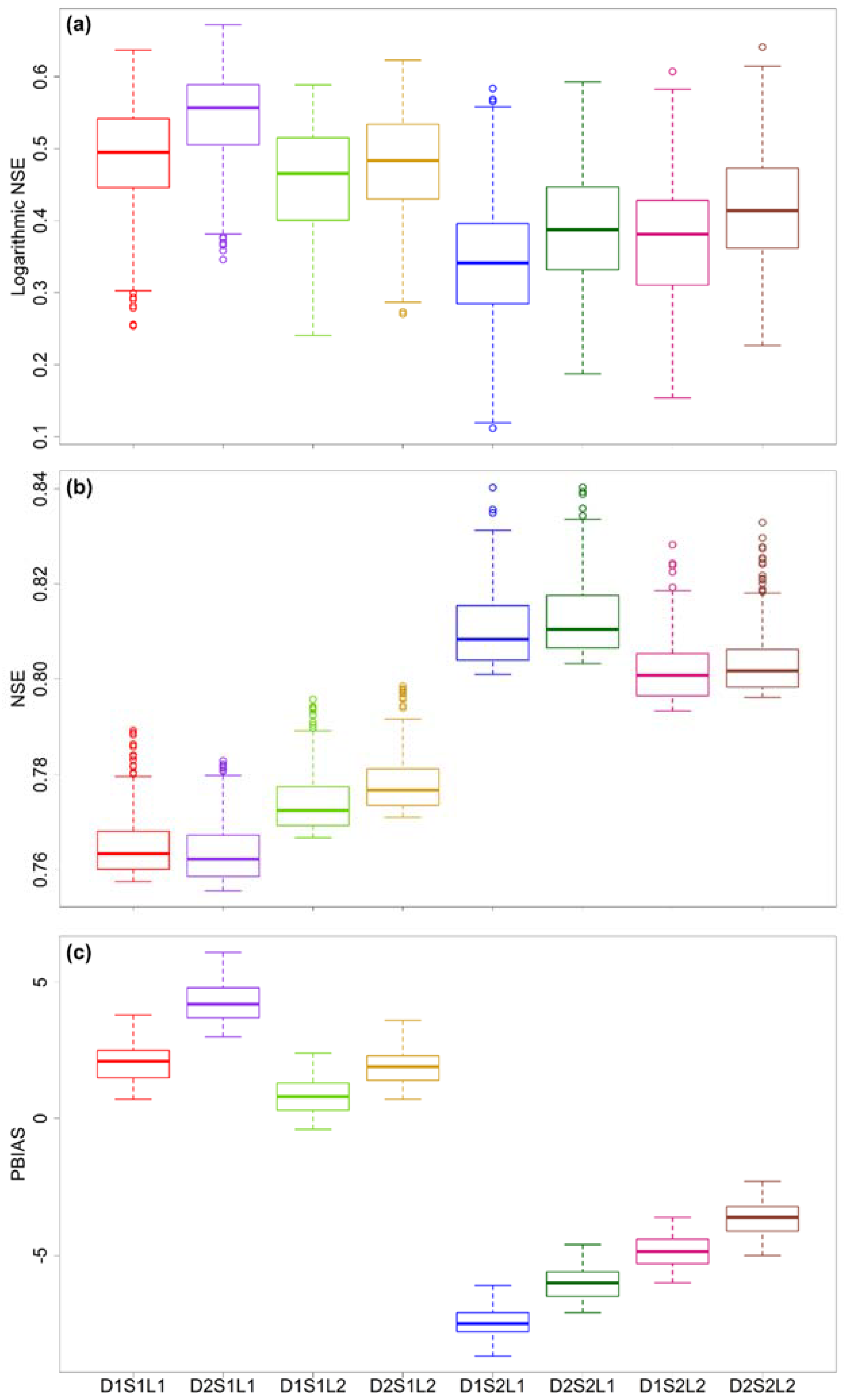
The model was calibrated using six parameters described in Table 2. We focused on the parameters that are not directly affected by soil, LULC, or topographic information to facilitate the evaluation of the effects of the various spatial products. Our Bayesian calibration resulted in the formation of two groups driven by the different information content of the soil maps, S1 and S2 (Figure 3).
The NSE values range from 0.76 to 0.82 (Figure 3b), indicating a good performance for all model setups. The small variances among NSEs indicate that high flows are not very sensitive to the differences between the various investigated spatial input data. However, a more-detailed soil map (S2) results in higher NSEs and generates a better representation of high flows/events. The main difference between soil maps S1 and S2 is the soil depth, which is important information for a hydrological model to estimate storage volume and retention time of the water [71]. Gatzke et al. [72] and Ficklin et al. [73] agreed that variations in soil depths may be one of the main causes of differences in the hydrologic output for the SWAT model.
Log NSE values are substantially lower than NSE, varying between 0.28 and 0.59 (Figure 3a), and the log NSE value was greater than 0.5 for only one setup (D2S1L1). This may represent a structural model problem in representing low flows and, as suggested by Geza and McGray [74], it could indicate a bad prediction of base flow since that is dominant during low flow conditions. Furthermore, Gassman et al. [75] suggested that weak results can be attributed in part to inadequate representation of rainfall inputs. As we only had one rainfall gauging station available for our simulation, the model simulates a rainfall-runoff reaction with almost every rainfall input, contrasting the observations. This situation assumes uniformity of precipitation throughout the watershed, neglecting its spatial variability. When available, the use of multiple stations or radar could improve the model prediction [76,77,78]. Another possible explanation for the lack of fitting for low flows is the choice of the likelihood function that optimizes high flows more efficiently [68].
Taking a closer look at the log NSE distribution, setups using the regional DEM D2 present a slightly better performance than those using global DEM D1 (Figure 3a), suggesting a sensitivity to small topographic changes. However, these differences are not clear for high flows (Figure 3b), where D1S1L1 and D2S1L1 present reverse behavior for D1 versus D2 for the NSE. Overall, we conclude that the regional D2 product is superior in reproducing streamflow. Many studies agree on the streamflow sensitivity to changes of DEM. Focusing on resolution, Cotter et al. [28] and Chaubey et al. [29], demonstrated that different DEMs result in different watershed areas, stream networks, and slopes and that these characteristics interfere with streamflow prediction. Dixon and Earls [32] showed that a 90 m DEM and a resampled 90 m DEM from a 30 m DEM contributed to different accuracies when predicting streamflow, highlighting the differences in information content when dealing with DEMs with the same resolution. Li and Wong [79] concluded that lowering DEM resolution does not necessarily lead to a poor model performance with respect to the quality of the data source. However, they expressed some concern about assuming that derived lower-resolution data are always superior to another lower resolution from a different source.
Looking at the distribution of PBIAS values (Figure 3c), one can see that the more-detailed LULC map (L2) results in PBIAS values closer to zero, i.e., a slightly better representation of the overall water balance. Earlier findings confirmed that streamflow is not extremely sensitive to LULC source or resolution. Huang et al. [80] found slight differences in the simulated monthly and daily streamflow when using three different LULC maps, in time, and in number of categories. After comparing seven resolutions of the same LULC map, Cotter et al. [28] showed that streamflow is not significantly affected by LULC resolution. By contrast, Tang et al. [81] investigated afforestation measures, which reduced modeled streamflow with SWAT. However, since our LULC maps mainly differed in pasture and agricultural categories we argue that these two LULC options do not effect evapotranspiration decisively, and thus the water balance of our catchment.
When combined with global soil map S1, setups using L2 presented a better model performance for high flows and a worse model performance for low flows than those using L1. However, the opposite is true when the setups are combined with the regional soil map S2, where L1 performs better than L2 for high flows and worse than L2 for low flows. PBIAS values also indicate that SWAT underestimates streamflow when using S1 and overestimates it when using S2. Despite indicating similar model performance for different soil maps, previous studies also indicated changes in the flow prediction. Cotter et al. [28] and Geza and McCray [74] suggested that decreases in soil map resolution may result in slower predicted flow. Wahren et al. [43] showed that soil maps with different data content may provide a different representation of the peak flow after a dry period.
3.2. Uncertainty Analysis
A reliable prediction model must be accurate, i.e., measure the bias representing how close the simulated values are to the observed data, and precise, i.e., representative of the range of the simulated values.
The simulation model accuracy is estimated in Figure 3 and represents its goodness-of-fit that was discussed in the previous section. Figure 3 also shows the simulation precision pictured as the width of each boxplot, which represents the model parameter uncertainty. All setups present similar uncertainties on the simulated discharge and a higher uncertainty for low flow predictions compared to high flow predictions.
Figure 4 represents the accuracy and precision of the simulation, showing the 95PPU in the hydrography, how much this interval bracket observed discharge data (P-factor), and how spread the simulated data are (R-factor). Notice that the P-factor indicates how much of the uncertainty we are capturing. All setups present similar P- and R-factor values, with the P-factor varying from 0.34 to 0.41 and the R-factor varying from 0.41 to 0.45. Confirming the difference shown in Figure 3, the hydrographs slightly differ depending on the use of different soil information, presenting smaller P-factors for S1 and greater for S2. These results agree with Shen et al. [48] and Kumar and Merwade [40] who showed a relative difference on prediction uncertainty, which could be due to the ranges of calibrated parameters.
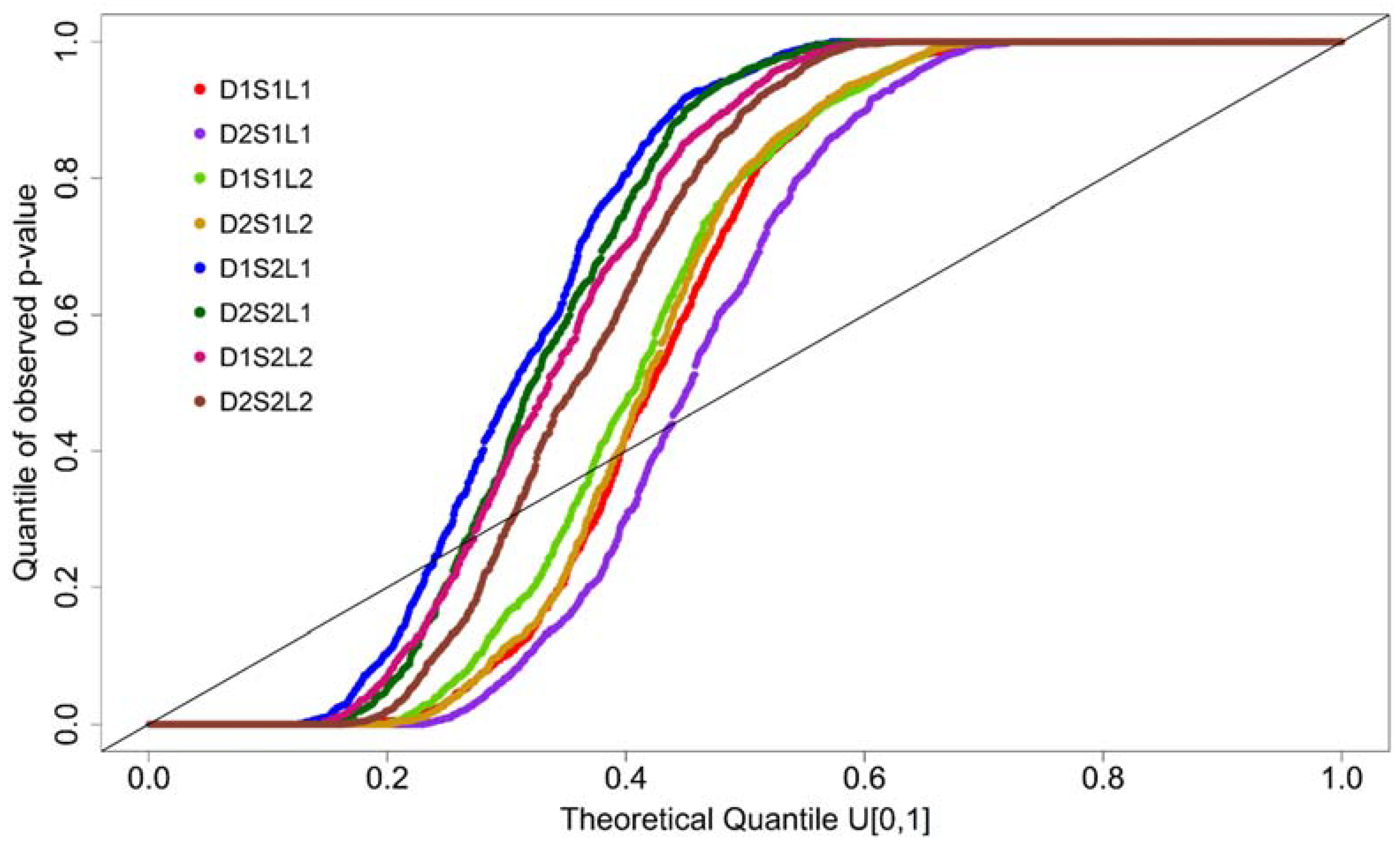
We use the quantile–quantile plot (QQ plot) adapted from the probabilistic forecast to evaluate the uncertainty analysis [13]. The predictive QQ plot compares the cumulative distribution function (cdf) of the simulated discharge to the cdf of a uniform distribution. Consequently, it is possible to assess whether the hypotheses in the calibration framework are consistent with the observed data by analyzing the relation between the QQ plot and the identity line. Figure 5 shows the QQ plot for all setups, and the curve shape suggests that these predictive uncertainties are being underestimated [13], which means that there are further uncertainties that are not considered in our modelling approach. As Leta et al. [82] showed, once all sources of uncertainty are not considered at the same time the parameters will compensate for this lack of information. This compensation is also observable in the posterior parameter distribution, which is described in the following section. To solve this issue, Ajami et al. [12] and Yen et al. [15] suggested the use of a framework, IBUNE (Integrated Bayesian Uncertainty Estimator) and IPEAT (Integrated Parameter Estimation and Uncertainty Analysis Tool) respectively, to account for major uncertainties sources, such as, parameter, input data and model structure uncertainty. However, both frameworks only consider precipitation as input data, not accounting for the uncertainty of spatial input data such as DEM, LULC and soil maps.
3.3. Posterior Parameter Distribution
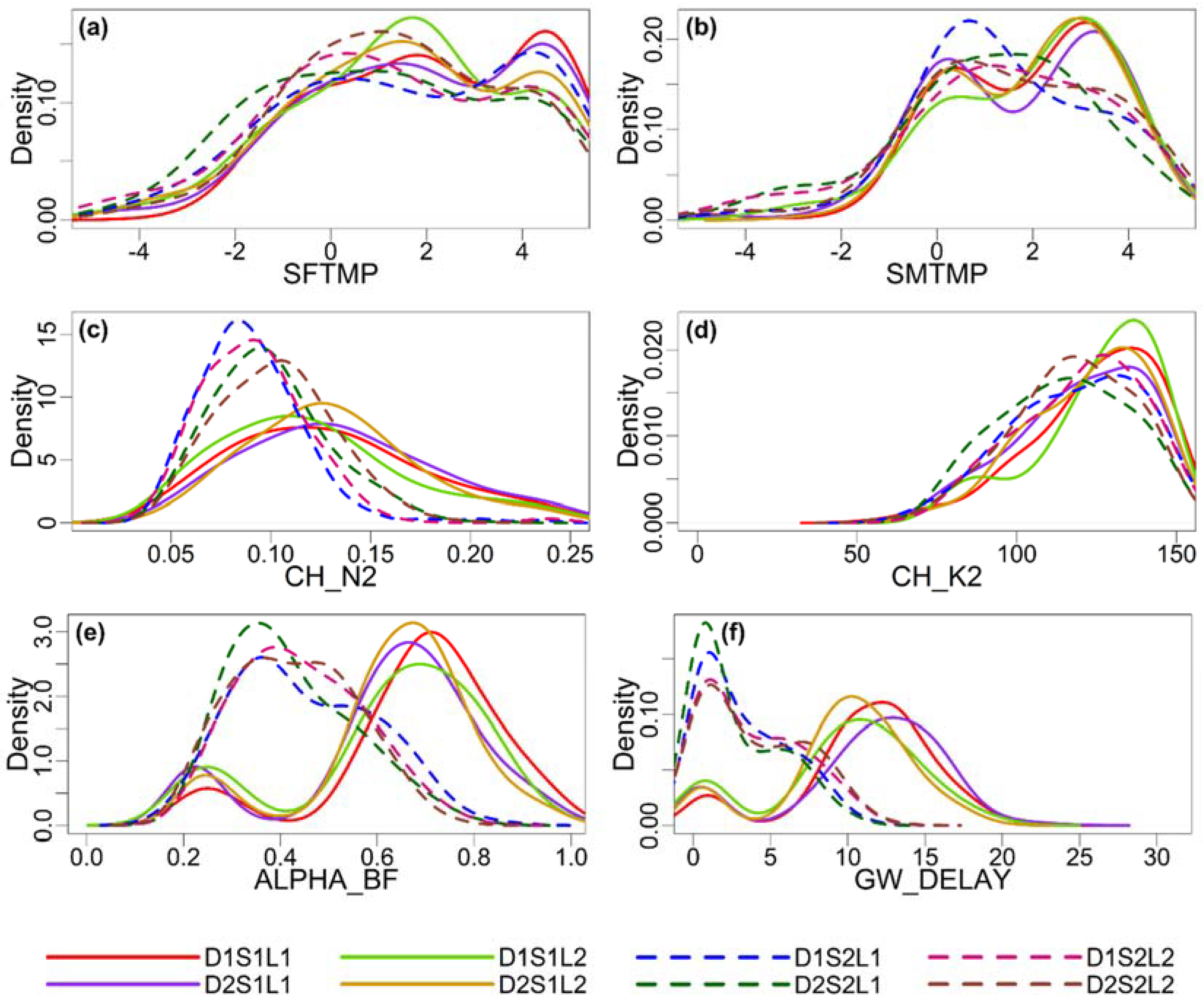
The parameter posterior distribution is shown in Figure 6. We noticed a constrained behavior for all calibrated parameters, highlighting the model sensitivity to these parameters. As with the pattern presented in the model efficiency criteria, the parameter posterior distribution separates into two groups with different parameters modal values, and these groups are driven by the soil information S1 and S2. All setups using S1 have similar parameter posterior distribution and are different from the parameter distributions for the S2 setups. Kumar and Merwade [40] and Bossa et al. [83] agree that despite presenting similar model performance, some parameters compensate for the differences in soil maps.
If the daily mean air temperature is less than the snowfall temperature model parameter (SFTMP), then the precipitation is classified as snow in the SWAT model. The corresponding amount of water is then rooted in a snow pack. The snow pack does not melt until its temperature exceeds the snow melt base temperature model parameter (SMTMP). Thereafter, the snowmelt is added to rainfall runoff and the percolation calculation [71]. SFTMP and SMTMP can vary between −5 and 5 °C. The posterior distributions show that
The SFTMP modal value varies between 0.1 and 4.5 (Figure 6a), and the modal SMTMP value varies between 0.6 for setups using S2 and 3.3 for setups using S1 (Figure 6b).
The Manning’s value for the main channel (CH_N2) is an empirical coefficient related to roughness, and it can vary between 0.01 and 0.25 mm h−1. The posterior distributions show a modal CH_N2 value varying between 0.11 and 0.12 for setups using S1 and between 0.08 and 0.10 for setups using S2 (Figure 6c). These values may represent “very weedy reaches, deep pools, or floodways with a heavy stand of timber and underbrush” [71].
Effective hydraulic conductivity in the main channel alluvium (CH_K2) describes the infiltration through the channel bottom and the higher its value, the higher the water loss rate from the river channel. CH_K2 can vary between 0.001 and 150 mm h−1. The posterior distribution shows that the CH_K2 model values vary between 134 and 136.6 for setups using S1 and are lower, between 116.6 and 131.3, for setups using S2 (Figure 6d). CH_K2 can be separated into groups according to the alluvium materials where high CH_K2 values, like those we obtained, correspond to an alluvium material formed by clean gravel and sand [71].
The base flow recession constant (Alpha_BF) is a direct index of groundwater flow response to changes in recharge [71,84]. Alpha_BF can vary between 0.001 and 0.99. The smaller its value, the slower the modeled land response to recharge is. Setups using S2 present a modal Alpha_BF value varying between 0.35 and 0.39, and setups using S1 present two peaks for the modal value of Alpha_BF, one between 0.22 and 0.25 and another between 0.67 and 0.71 (Figure 6e). Groundwater delay time (GW_delay) is the lag between the time that the water exits the soil profile and enters the shallow aquifer [71]. It can vary between 0 and 31 days, and dry regions with deep water tables may present long time delays. Posterior distributions show that GW_delay has two peaks for the modal value for each soil information: varying between 0.6–0.9 and 10.2–12.9 for S1 setups and between 0.8–1.1 and 5.3–7.0 for S2 setups (Figure 6f). The groundwater parameters are primordial for base flow prediction, a process that is dominant during low flow conditions. Our previous results showed that the model does not perform well for low flow events, which may explain the differences on groundwater parameters’ posterior distribution. These parameters are compensating for part of the model structure uncertainty.
4. Conclusions
This study builds on previous studies by others, which provided detailed insights into the use of different spatial input datasets. So far, a detailed intercomparison of DEM, LULC and soil maps was missing in order to address the influence of different spatial input datasets (DEM, LULC and soil maps) on SWAT performance estimating discharge and its uncertainty. Spatial data originating from different sources may provide different data content despite having the same resolution. We analyzed eight different setups using global (D1, L1, and S1) and regional (D2, L2, and S2) DEM, LULC, and soil maps.
Similar to previous studies by Chaubey et al. [29] who investigated DEM in different resolution and Yen et al. [35] who studied the effect of different land-use maps, our results indicate that the choice of regional or global information may depend on the focus of the analysis, because SWAT performance varies for high and low flows. SWAT predicted high flows efficiently for all setups, suggesting that the model is minimally affected by spatial input data differences for high flows. However, there is a notable difference among the setups when predicting low flows. When comparing all setups, those using the regional D2 and the global S1 are always more efficient in representing low flows, suggesting that SWAT is either sensitive to small topographic changes but cannot necessarily make use of additional soil information, or that there are other model errors that we have not considered. The model setup D2S1L1 represents the only setup with a log NSE greater than 0.5, indicating that additional data or missing processes are needed to improve the model’s capability to simulate low flows in this catchment.
Each parameter presents a similar posterior distribution according to the soil map used, indicating smaller parameter values for the setups using the regional S2 map. Additionally, there is a constrained behavior of all parameter posterior distributions for all setups, highlighting the model sensitivity to these parameters. All setups present similar uncertainty on the output and higher uncertainty for low-flow than for high-flow predictions. Furthermore, the QQ plot results show that all model setups underestimate the model uncertainty, suggesting that additional sources of uncertainties should be considered simultaneously. To proceed further in addressing all sources of modelling uncertainty, one promising way forward would be to combine our methodology with the work presented by [12,15] with their IPEAT and IBUNE frameworks in order to account for meteorological input data and model structure uncertainty.
Author Contributions
C.C. performed the calculations, analyzed the results and wrote the paper; S.J. provided expertise on SWAT, supervised the model setup and provided expertise on the area of study; T.H. developed the parameter estimation tool, supervised the work and contributed to the paper writing; M.B. contributed to the paper writing; L.B. provided the general idea of this paper, supervised the work and contributed to the paper writing.
Acknowledgments
This research was carried out as part of the Framework Marie Skłodowska Curie ITN—Quantifying Uncertainty in Integrated Catchment Studies (QUICS). QUICS has received funding from the European Union’s Seventh Framework Programme for research, technological development, and demonstration under grant agreement No. 607000. The Hessian Competence Center for High-Performance Computing (HKHLR) is acknowledged for the access provided for the use of the computer cluster.
Conflicts of Interest
The authors declare no conflict of interest.
References
- Jimenez Cisneros, B.E.; Oki, T.; Arnell, N.W.; Benito, G.; Cogley, J.G.; Doll, P.; Jiang, T.; Mwakalila, S.S. Freshwater resources. In Climate Change 2014: Impacts, Adaptation and Vulnerability. Part A: Global and Sectoral Aspects. Contribution of Working Group II to the Fifth Assessment Report of the Intergovernmental Panel on Climate Change; Field, C.B., Barros, V.R., Dokken, D.J., Mach, K.J., Mastrandrea, M.D., Bilir, T.E., Chatterjee, M., Ebi, K.L., Estrada, Y.O., Genova, R.C., et al., Eds.; Cambridge University Press: Cambridge, UK, 2014; pp. 229–269. [Google Scholar]
- Hall, J.; Arheimer, B.; Borga, M.; Brázdil, R.; Claps, P.; Kiss, A.; Kjeldsen, T.R.; Kriauciuniene, J.; Kundzewicz, Z.W.; Lang, M.; et al. Understanding Flood Regime Changes in Europe: A state of the art assessment. Hydrol. Earth Syst. Sci. 2014, 18, 2735–2772. [Google Scholar] [CrossRef] [Green Version]
- Barnett, T.P.; Pierce, D.W.; Hidalgo, H.G.; Bonfils, C.; Santer, B.D.; Das, T.; Bala, G.; Wood, A.W.; Nozawa, T.; Mirin, A.A.; et al. Human-Induced Changes in the Hydrology of the Western United States. Science 2008, 319, 1080–1083. [Google Scholar] [CrossRef] [PubMed]
- Reed, S.; Koren, V.; Smith, M.; Zhang, Z.; Moreda, F.; Seo, D.-J.; DMIP Participants. Overall distributed model intercomparison project results. J. Hydrol. 2004, 298, 27–60. [Google Scholar] [CrossRef]
- Breuer, L.; Huisman, J.A.; Willems, P.; Bormann, H.; Bronstert, A.; Croke, B.F.W.; Frede, H.-G.; Gräff, T.; Hubrechts, L.; Jakeman, A.J.; et al. Assessing the impact of land use change on hydrology by ensemble modeling (LUCHEM). I: Model intercomparison with current land use. Adv. Water Resour. 2009, 32, 129–146. [Google Scholar] [CrossRef]
- Smith, M.B.; Koren, V.; Reed, S.; Zhang, Z.; Zhang, Y.; Moreda, F.; Cui, Z.; Mizukami, N.; Anderson, E.A.; Cosgrove, B.A. The distributed model intercomparison project—Phase 2: Motivation and design of the Oklahoma experiments. J. Hydrol. 2012, 418–419, 3–16. [Google Scholar] [CrossRef]
- Krysanova, V.; Vetter, T.; Eisner, S.; Huang, S.; Pechlivanidis, I.; Michael, S.; Gelfan, A.; Kumar, R.; Aich, V.; Arheimer, B.; et al. Intercomparison of regional-scale hydrological models and climate change impacts projected for 12 large river basins worldwide—A synthesis. Environ. Res. Lett. 2017, 12, 105002. [Google Scholar] [CrossRef]
- Refsgaard, J.C.; van der Sluijs, J.P.; Højberg, A.L.; Vanrolleghem, P.A. Uncertainty in the environmental modelling process—A framework and guidance. Environ. Model. Softw. 2007, 22, 1543–1556. [Google Scholar] [CrossRef]
- Beven, K.; Binley, A. The future of distributed models: Model calibration and uncertainty prediction. Hydrol. Process. 1992, 6, 279–298. [Google Scholar] [CrossRef]
- Legates, D.R.; McCabe, G.J. Evaluating the use of “goodness-of-fit” measures in hydrologic and hydroclimatic model validation. Water Resour. Res. 1999, 35, 233–241. [Google Scholar] [CrossRef]
- Refsgaard, J.C.; van der Sluijs, J.P.; Brown, J.; van der Keur, P. A framework for dealing with uncertainty due to model structure error. Adv. Water Resour. 2006, 29, 1586–1597. [Google Scholar] [CrossRef]
- Ajami, N.; Duan, Q.; Sorooshian, S. An integrated hydrologic Bayesian multimodel combination framework: Confronting input, parameter, and model structural uncertainty in hydrologic prediction. Water Resour. Res. 2007, 43. [Google Scholar] [CrossRef]
- Thyer, M.; Renard, B.; Kavetski, D.; Kuczera, G.; Franks, S.W.; Srikanthan, S. Critical evaluation of parameter consistency and predictive uncertainty in hydrological modeling: A case study using Bayesian total error analysis: PARAMETER CONSISTENCY AND PREDICTIVE UNCERTAINTY. Water Resour. Res. 2009, 45. [Google Scholar] [CrossRef]
- McMillan, H.; Krueger, T.; Freer, J. Benchmarking observational uncertainties for hydrology: Rainfall, river discharge and water quality. Hydrol. Process. 2012, 26, 4078–4111. [Google Scholar] [CrossRef]
- Yen, H.; Wang, X.; Fontane, D.G.; Harmel, R.D.; Arabi, M. A framework for propagation of uncertainty contributed by parameterization, input data, model structure, and calibration/validation data in watershed modeling. Environ. Model. Softw. 2014, 54, 211–221. [Google Scholar] [CrossRef]
- Wani, O.; Scheidegger, A.; Carbajal, J.P.; Rieckermann, J.; Blumensaat, F. Parameter estimation of hydrologic models using a likelihood function for censored and binary observations. Water Res. 2017, 121, 290–301. [Google Scholar] [CrossRef] [PubMed]
- Sharma, A.; Tiwari, K.N. A comparative appraisal of hydrological behavior of SRTM DEM at catchment level. J. Hydrol. 2014, 519, 1394–1404. [Google Scholar] [CrossRef]
- Wang, H.; Wu, Z.; Hu, C. A Comprehensive Study of the Effect of Input Data on Hydrology and non-point Source Pollution Modeling. Water Resour. Manag. 2015, 29, 1505–1521. [Google Scholar] [CrossRef]
- Vrugt, J.A.; ter Braak, C.J.F.; Clark, M.P.; Hyman, J.M.; Robinson, B.A. Treatment of input uncertainty in hydrologic modeling: Doing hydrology backward with Markov chain Monte Carlo simulation: FORCING DATA ERROR USING MCMC SAMPLING. Water Resour. Res. 2008, 44. [Google Scholar] [CrossRef]
- Beven, K. Facets of uncertainty: Epistemic uncertainty, non-stationarity, likelihood, hypothesis testing, and communication. Hydrol. Sci. J. 2016, 61, 1652–1665. [Google Scholar] [CrossRef]
- Bormann, H.; Breuer, L.; Gräff, T.; Huisman, J.A.; Croke, B. Assessing the impact of land use change on hydrology by ensemble modelling (LUCHEM) IV: Model sensitivity to data aggregation and spatial (re-)distribution. Adv. Water Resour. 2009, 32, 171–192. [Google Scholar] [CrossRef]
- Bastola, S.; Murphy, C.; Sweeney, J. The role of hydrological modelling uncertainties in climate change impact assessments of Irish river catchments. Adv. Water Resour. 2011, 34, 562–576. [Google Scholar] [CrossRef]
- Najafi, M.R.; Moradkhani, H.; Jung, I.W. Assessing the uncertainties of hydrologic model selection in climate change impact studies. Hydrol. Process. 2011, 25, 2814–2826. [Google Scholar] [CrossRef]
- Exbrayat, J.-F.; Buytaert, W.; Timbe, E.; Windhorst, D.; Breuer, L. Addressing sources of uncertainty in runoff projections for a data scarce catchment in the Ecuadorian Andes. Clim. Chang. 2014, 125, 221–235. [Google Scholar] [CrossRef]
- Breuer, L.; Vaché, K.B.; Julich, S.; Frede, H.-G. Current concepts in nitrogen dynamics for mesoscale catchments. Hydrol. Sci. J. 2008, 53, 1059–1074. [Google Scholar] [CrossRef]
- Arnold, J.G.; Srinivasan, R.; Muttiah, R.S.; Williams, J.R. Large area hydrologic modeling and assessment part I: Model development. J. Am. Water Resour. Assoc. 1998, 34, 73–89. [Google Scholar] [CrossRef]
- Chaplot, V. Impact of spatial input data resolution on hydrological and erosion modeling: Recommendations from a global assessment. Phys. Chem. Earth Parts ABC 2014, 67–69, 23–35. [Google Scholar] [CrossRef]
- Cotter, A.S.; Chaubey, I.; Costello, T.A.; Soerens, T.S.; Nelson, M.A. Water Quality Model Output Uncertainty as Affected by Spatial Resolution of Input Data. J. Am. Water Resour. Assoc. 2003, 39, 977–986. [Google Scholar] [CrossRef]
- Chaubey, I.; Cotter, A.S.; Costello, T.A.; Soerens, T.S. Effect of DEM data resolution on SWAT output uncertainty. Hydrol. Process. 2005, 19, 621–628. [Google Scholar] [CrossRef]
- Tan, M.L.; Ficklin, D.L.; Dixon, B.; Ibrahim, A.L.; Yusop, Z.; Chaplot, V. Impacts of DEM resolution, source, and resampling technique on SWAT-simulated streamflow. Appl. Geogr. 2015, 63, 357–368. [Google Scholar] [CrossRef]
- Lin, S.; Jing, C.; Coles, N.A.; Chaplot, V.; Moore, N.J.; Wu, J. Evaluating DEM source and resolution uncertainties in the Soil and Water Assessment Tool. Stoch. Environ. Res. Risk Assess. 2013, 27, 209–221. [Google Scholar] [CrossRef]
- Dixon, B.; Earls, J. Resample or not?! Effects of resolution of DEMs in watershed modeling. Hydrol. Process. 2009, 23, 1714–1724. [Google Scholar] [CrossRef]
- Zhang, P.; Liu, R.; Bao, Y.; Wang, J.; Yu, W.; Shen, Z. Uncertainty of SWAT model at different DEM resolutions in a large mountainous watershed. Water Res. 2014, 53, 132–144. [Google Scholar] [CrossRef] [PubMed]
- Xu, F.; Dong, G.; Wang, Q.; Liu, L.; Yu, W.; Men, C.; Liu, R. Impacts of DEM uncertainties on critical source areas identification for non-point source pollution control based on SWAT model. J. Hydrol. 2016, 540, 355–367. [Google Scholar] [CrossRef]
- Yen, H.; Sharifi, A.; Kalin, L.; Mirhosseini, G.; Arnold, J.G. Assessment of model predictions and parameter transferability by alternative land use data on watershed modeling. J. Hydrol. 2015, 527, 458–470. [Google Scholar] [CrossRef]
- Asante, K.; Leh, M.D.; Cothren, J.D.; Luzio, M.D.; Brahana, J.V. Effects of land-use land-cover data resolution and classification methods on SWAT model flow predictive reliability. Int. J. Hydrol. Sci. Technol. 2016, 7, 39–62. [Google Scholar] [CrossRef]
- Pai, N.; Saraswat, D. Impact of land use and land cover categorical uncertainty on SWAT hydrologic modeling. Trans. ASABE 2013, 56, 1387–1397. [Google Scholar] [CrossRef]
- El-Sadek, A.; İrvem, A. Evaluating the impact of land use uncertainty on the simulated streamflow and sediment yield of the Seyhan River basin using the SWAT model. Turk. J. Agric. For. 2014, 38, 515–530. [Google Scholar] [CrossRef]
- Chen, L.; Wang, G.; Zhong, Y.; Shen, Z. Evaluating the impacts of soil data on hydrological and nonpoint source pollution prediction. Sci. Total Environ. 2016, 563–564, 19–28. [Google Scholar] [CrossRef] [PubMed]
- Kumar, S.; Merwade, V. Impact of Watershed Subdivision and Soil Data Resolution on SWAT Model Calibration and Parameter Uncertainty. J. Am. Water Resour. Assoc. 2009, 45, 1179–1196. [Google Scholar] [CrossRef]
- Heathman, G.C.; Larose, M.; Ascough, J.C. Soil and Water Assessment Tool evaluation of soil and land use geographic information system data sets on simulated stream flow. J. Soil Water Conserv. 2009, 64, 17–32. [Google Scholar] [CrossRef]
- Moriasi, D.N.; Starks, P.J. Effects of the resolution of soil dataset and precipitation dataset on SWAT2005 streamflow calibration parameters and simulation accuracy. J. Soil Water Conserv. 2010, 65, 63–78. [Google Scholar] [CrossRef]
- Tavares Wahren, F.; Julich, S.; Nunes, J.P.; Gonzalez-Pelayo, O.; Hawtree, D.; Feger, K.-H.; Keizer, J.J. Combining digital soil mapping and hydrological modeling in a data scarce watershed in north-central Portugal. Geoderma 2016, 264, 350–362. [Google Scholar] [CrossRef]
- Renard, B.; Kavetski, D.; Kuczera, G.; Thyer, M.; Franks, S.W. Understanding predictive uncertainty in hydrologic modeling: The challenge of identifying input and structural errors. Water Resour. Res. 2010, 46. [Google Scholar] [CrossRef] [Green Version]
- Hargreaves, G.L.; Hargreaves, G.H.; Riley, J.P. Agricultural benefits for Senegal River basin. J. Irrig. Drain. Eng. 1985, 111, 113–124. [Google Scholar] [CrossRef]
- Digital Elevation Model over Europe (EU-DEM). Available online: https://www.eea.europa.eu/data-and-maps/data/eu-dem (accessed on 7 November 2017).
- EU-DEM Statistical Validation Report. Available online: http://ec.europa.eu/eurostat/documents/4311134/4350046/Report-EU-DEM-statistical-validation-August2014.pdf/508200d9-b52d-4562-b73b-edb64eedfb93 (accessed on 7 November 2017).
- Shen, Z.Y.; Chen, L.; Liao, Q.; Liu, R.M.; Huang, Q. A comprehensive study of the effect of GIS data on hydrology and non-point source pollution modeling. Agric. Water Manag. 2013, 118, 93–102. [Google Scholar] [CrossRef]
- Chaplot, V. Impact of DEM mesh size and soil map scale on SWAT runoff, sediment, and NO3–N loads predictions. J. Hydrol. 2005, 312, 207–222. [Google Scholar] [CrossRef]
- Wu, M.; Shi, P.; Chen, A.; Shen, C.; Wang, P. Impacts of DEM resolution and area threshold value uncertainty on the drainage network derived using SWAT. Water SA 2017, 43, 450–462. [Google Scholar] [CrossRef]
- Eckelmann, W.; Sponagel, H.; Grottenthaler, W.; Hartmann, K.-J.; Hartwich, R.; Janetzko, P.; Joisten, H.; Kühn, D.; Sabel, K.-J.; Traidl, R. Bodenkundliche Kartieranleitung. KA5; Schweizerbart Science Publishers: Stuttgart, Germany, 2006; ISBN 978-3-510-95920-4. [Google Scholar]
- CLC 2006—Copernicus Land Monitoring Service. Available online: https://land.copernicus.eu/pan-european/corine-land-cover/clc-2006 (accessed on 8 February 2018).
- Nachtergaele, F.O.; van Velthuizen, H.; Verelst, L.; Wiberg, D. Harmonized World Soil Database (Version 1.2); Food and Agric Organization of the UN (FAO); International Inst. for Applied Systems Analysis (IIASA); ISRIC-World Soil Information; Inst of Soil Science-Chinese Acad of Sciences (ISS-CAS); EC-Joint Research Centre (JRC); FAO: Rome, Italy; IIASA: Laxenburg, Austria, 2012. [Google Scholar]
- Hengl, T.; de Jesus, J.M.; Heuvelink, G.B.; Gonzalez, M.R.; Kilibarda, M.; Blagotić, A.; Shangguan, W.; Wright, M.N.; Geng, X.; Bauer-Marschallinger, B.; et al. SoilGrids250m: Global gridded soil information based on machine learning. PLoS ONE 2017, 12, e0169748. [Google Scholar] [CrossRef] [PubMed]
- Saxton, K.E.; Rawls, W.J. Soil Water Characteristic Estimates by Texture and Organic Matter for Hydrologic Solutions. Soil Sci. Soc. Am. J. 2006, 70, 1569–1578. [Google Scholar] [CrossRef]
- Flanagan, D.C.; Livingston, S.J. WEPP User Summary: USDA-Water Erosion Prediction Project (WEPP); National Soil Erosion Research Laboratory, USDA-ARS-MWA: West Lafayette, IN, USA, 1995.
- Metropolis, N.; Rosenbluth, A.W.; Rosenbluth, M.N.; Teller, A.H.; Teller, E. Equation of State Calculations by Fast Computing Machines. J. Chem. Phys. 1953, 21, 1087–1092. [Google Scholar] [CrossRef]
- Houska, T.; Kraft, P.; Chamorro-Chavez, A.; Breuer, L. SPOTting Model Parameters Using a Ready-Made Python Package. PLoS ONE 2015, 10, e0145180. [Google Scholar] [CrossRef] [PubMed]
- White, K.L.; Chaubey, I. Sensitivity Analysis, Calibration, and Validations for a Multisite and Multivariable Swat Model1. J. Am. Water Resour. Assoc. 2005, 41, 1077–1089. [Google Scholar] [CrossRef]
- Arnold, J.G.; Moriasi, D.N.; Gassman, P.W.; Abbaspour, K.C.; White, M.J.; Srinivasan, R.; Santhi, C.; Harmel, R.D.; Van Griensven, A.; Van Liew, M.W.; et al. SWAT: Model use, calibration, and validation. Trans. ASABE 2012, 55, 1491–1508. [Google Scholar] [CrossRef]
- Abbaspour, K.C.; Rouholahnejad, E.; Vaghefi, S.; Srinivasan, R.; Yang, H.; Kløve, B. A continental-scale hydrology and water quality model for Europe: Calibration and uncertainty of a high-resolution large-scale SWAT model. J. Hydrol. 2015, 524, 733–752. [Google Scholar] [CrossRef]
- Vrugt, J.A. Markov chain Monte Carlo simulation using the DREAM software package: Theory, concepts, and MATLAB implementation. Environ. Model. Softw. 2016, 75, 273–316. [Google Scholar] [CrossRef]
- Brooks, S.P.; Gelman, A. General methods for monitoring convergence of iterative simulations. J. Comput. Graph. Stat. 1998, 7, 434–455. [Google Scholar] [CrossRef]
- Nash, J.E.; Sutcliffe, J.V. River flow forecasting through conceptual models part I—A discussion of principles. J. Hydrol. 1970, 10, 282–290. [Google Scholar] [CrossRef]
- Moriasi, D.N.; Arnold, J.G.; van Liew, M.W.; Bingner, R.L.; Harmel, R.D.; Veith, T.L. Model Evaluation Guidelines for Systematic Quantification of Accuracy in Watershed Simulations. Trans. ASABE 2007, 50, 885–900. [Google Scholar] [CrossRef]
- Krause, P.; Boyle, D.P.; Bäse, F. Comparison of different efficiency criteria for hydrological model assessment. Adv. Geosci. 2005, 5, 89–97. [Google Scholar] [CrossRef]
- Oudin, L.; Andréassian, V.; Mathevet, T.; Perrin, C.; Michel, C. Dynamic averaging of rainfall-runoff model simulations from complementary model parameterizations. Water Resour. Res. 2006, 42, W07410. [Google Scholar] [CrossRef]
- Pushpalatha, R.; Perrin, C.; Moine, N.L.; Andréassian, V. A review of efficiency criteria suitable for evaluating low-flow simulations. J. Hydrol. 2012, 420–421, 171–182. [Google Scholar] [CrossRef]
- Gupta, H.V.; Sorooshian, S.; Yapo, P.O. Status of Automatic Calibration for Hydrologic Models: Comparison with Multilevel Expert Calibration. J. Hydrol. Eng. 1999, 4, 135–143. [Google Scholar] [CrossRef]
- Abbaspour, K.C.; Yang, J.; Maximov, I.; Siber, R.; Bogner, K.; Mieleitner, J.; Zobrist, J.; Srinivasan, R. Modelling hydrology and water quality in the pre-alpine/alpine Thur watershed using SWAT. J. Hydrol. 2007, 333, 413–430. [Google Scholar] [CrossRef]
- Arnold, J.G.; Kiniry, J.R.; Srinivasan, R.; Williams, J.R.; Haney, E.B.; Neitsch, S.L. SWAT 2012 Input/Output Documentation; Texas Water Resources Institute: College Station, TX, USA, 2013. [Google Scholar]
- Gatzke, S.E.; Beaudette, D.E.; Ficklin, D.L.; Luo, Y.; O’Geen, A.T.; Zhang, M. Aggregation Strategies for SSURGO Data: Effects on SWAT Soil Inputs and Hydrologic Outputs. Soil Sci. Soc. Am. J. 2011, 75, 1908–1921. [Google Scholar] [CrossRef]
- Ficklin, D.L.; Luo, Y.; Zhang, M.; Gatzke, S.E. The use of soil taxonomy as a soil type identifier for the Shasta Lake Watershed using SWAT. Trans. ASABE 2014, 57, 717–728. [Google Scholar] [CrossRef]
- Geza, M.; McCray, J.E. Effects of soil data resolution on SWAT model stream flow and water quality predictions. J. Environ. Manag. 2008, 88, 393–406. [Google Scholar] [CrossRef] [PubMed]
- Gassman, P.W.; Reyes, M.R.; Green, C.H.; Arnold, J.G. The soil and water assessment tool: Historical development, applications, and future research directions. Trans. ASABE 2007, 50, 1211–1250. [Google Scholar] [CrossRef]
- Chaplot, V.; Saleh, A.; Jaynes, D.B. Effect of the accuracy of spatial rainfall information on the modeling of water, sediment, and NO3–N loads at the watershed level. J. Hydrol. 2005, 312, 223–234. [Google Scholar] [CrossRef]
- Muleta, M.K.; Nicklow, J.W.; Bekele, E.G. Sensitivity of a distributed watershed simulation model to spatial scale. J. Hydrol. Eng. 2007, 12, 163–172. [Google Scholar] [CrossRef]
- Cho, J.; Bosch, D.; Lowrance, R.; Strickland, T.; Vellidis, G. Effect of Spatial Distribution of Rainfall on Temporal and Spatial Uncertainty of SWAT Output. Trans. ASABE 2009, 52, 1545–1556. [Google Scholar] [CrossRef]
- Li, J.; Wong, D.W.S. Effects of DEM sources on hydrologic applications. Comput. Environ. Urban Syst. 2010, 34, 251–261. [Google Scholar] [CrossRef]
- Huang, J.; Zhou, P.; Zhou, Z.; Huang, Y. Assessing the Influence of Land Use and Land Cover Datasets with Different Points in Time and Levels of Detail on Watershed Modeling in the North River Watershed, China. Int. J. Environ. Res. Public Health 2013, 10, 144–157. [Google Scholar] [CrossRef] [PubMed]
- Tang, L.; Yang, D.; Hu, H.; Gao, B. Detecting the effect of land-use change on streamflow, sediment and nutrient losses by distributed hydrological simulation. J. Hydrol. 2011, 409, 172–182. [Google Scholar] [CrossRef]
- Leta, O.T.; Nossent, J.; Velez, C.; Shrestha, N.K.; van Griensven, A.; Bauwens, W. Assessment of the different sources of uncertainty in a SWAT model of the River Senne (Belgium). Environ. Model. Softw. 2015, 68, 129–146. [Google Scholar] [CrossRef]
- Bossa, A.Y.; Diekkrüger, B.; Igué, A.M.; Gaiser, T. Analyzing the effects of different soil databases on modeling of hydrological processes and sediment yield in Benin (West Africa). Geoderma 2012, 173–174, 61–74. [Google Scholar] [CrossRef]
- Smedema, L.K.; Rycroft, D.W. Land Drainage: Planning and Design of Agricultural Systems; Cornell University Press: Ithaca, NY, USA, 1983. [Google Scholar]
Figure 1.
The study area location with its stream network. Meteorological conditions are measured in a daily resolution next to Schimpach, Luxembourg (50°00′36′′ E, 5°50′56′′ N), while the discharge of the Wiltz River is measured at the outlet close to the city of Winseler (49°58′04′′ E, 5°53′23′′ N).

Figure 2.
Regional and global datasets for the study area: digital elevation model (DEM), soil, and land use/land cover (LULC) maps. Detailed input data maps (D2, S2, and L2) are compared with global maps (D1, S1, and L1) and cross-combined into eight different model setups.
Figure 2.
Regional and global datasets for the study area: digital elevation model (DEM), soil, and land use/land cover (LULC) maps. Detailed input data maps (D2, S2, and L2) are compared with global maps (D1, S1, and L1) and cross-combined into eight different model setups.

Figure 3.
Posterior SWAT performance results after Bayesian calibration with the Markov Chain Monte Carlo (MCMC) algorithm, evaluated for different goodness-of-fit functions. The top panel (a) shows the posterior log Nash–Sutcliffe Efficiency (NSE) results in fitting the discharge observation, the middle panel (b) shows the NSE and the bottom panel (c) shows the percent bias (PBIAS). The X-axis shows the model setups.

Figure 4.
Hydrographs comparing all setups (a–h), including the 95% prediction uncertainty and the P- and R-factors.
Figure 4.
Hydrographs comparing all setups (a–h), including the 95% prediction uncertainty and the P- and R-factors.

Figure 5.
Predictive quantile–quantile (QQ) plots of the different best fit model SWAT setups derived from different input data (see Table 1).
Figure 5.
Predictive quantile–quantile (QQ) plots of the different best fit model SWAT setups derived from different input data (see Table 1).

Figure 6.
Density curves representing the posterior parameter distribution (a–f) for all tested SWAT model setups (see Table 2 for acronyms and definition of model parameters). The different model setup combinations refer to digital elevation maps (D), LULC maps (L) and soil maps (S) (see Table 1 for further description). Results are grouped by the use of a global soil map (S1) with a solid line and a regional soil map (S2) as a dashed line.


Table 1.
Model setups used in the analysis.
| Model Setup | Number of Subbasins | Number of HRUs | Watershed Area (km2) | Stream Network Length (km) |
|---|---|---|---|---|
| D1S1L1 | 8 | 90 | 103.0 | 33.5 |
| D2S1L1 | 8 | 89 | 104.2 | 33.0 |
| D1S1L2 | 8 | 99 | 103.0 | 33.5 |
| D2S1L2 | 8 | 100 | 104.2 | 33.0 |
| D1S2L1 | 8 | 173 | 103.0 | 33.5 |
| D2S2L1 | 8 | 174 | 104.2 | 33.0 |
| D1S2L2 | 8 | 199 | 103.0 | 33.5 |
| D2S2L2 | 8 | 200 | 104.2 | 33.0 |
Table 2.
Parameters’ name, description, and units, default value on Soil and Water Assessment Tool (SWAT) and range used for prior distribution.
Table 2.
Parameters’ name, description, and units, default value on Soil and Water Assessment Tool (SWAT) and range used for prior distribution.
| Parameter Name | Parameter Definition | Parameter Factor | SWAT Default | Prior lower Bound | Prior Upper Bound | Units |
|---|---|---|---|---|---|---|
| SFTMP | Snowfall temperature | Replace | 1 | −5 | 5 | °C |
| SMTMP | Snowmelt base temperature | Replace | 0.5 | −5 | 5 | °C |
| CHN | Manning’s roughness coefficient, n | Replace | 0.014 | 0.01 | 0.25 | mm h−1 |
| CHK | Hydraulic conductivity of channel | Replace | 0 | 0.001 | 150 | mm h−1 |
| ALPHA_BF | Base flow alpha factor | Replace | 0.048 | 0.001 | 0.99 | - |
| GW_DELAY | Groundwater delay time | Replace | 31 | 0 | 31 | days |
© 2018 by the authors. Licensee MDPI, Basel, Switzerland. This article is an open access article distributed under the terms and conditions of the Creative Commons Attribution (CC BY) license (http://creativecommons.org/licenses/by/4.0/).
Share and Cite
MDPI and ACS Style
Camargos, C.; Julich, S.; Houska, T.; Bach, M.; Breuer, L. Effects of Input Data Content on the Uncertainty of Simulating Water Resources. Water 2018, 10, 621. https://doi.org/10.3390/w10050621
AMA Style
Camargos C, Julich S, Houska T, Bach M, Breuer L. Effects of Input Data Content on the Uncertainty of Simulating Water Resources. Water. 2018; 10(5):621. https://doi.org/10.3390/w10050621
Chicago/Turabian StyleCamargos, Carla, Stefan Julich, Tobias Houska, Martin Bach, and Lutz Breuer. 2018. "Effects of Input Data Content on the Uncertainty of Simulating Water Resources" Water 10, no. 5: 621. https://doi.org/10.3390/w10050621
Note that from the first issue of 2016, this journal uses article numbers instead of page numbers. See further details here.