Physical Hybrid Neural Network Model to Forecast Typhoon Floods

1
Construction and Disaster Prevention Research Center, Feng Chia University, Taichung 407, Taiwan
2
Department of Water Resources Engineering and Conservation, Feng Chia University, Taichung 407, Taiwan
*
Author to whom correspondence should be addressed.
Water 2018, 10(5), 632; https://doi.org/10.3390/w10050632
Submission received: 10 April 2018
/
Revised: 4 May 2018
/
Accepted: 10 May 2018
/
Published: 13 May 2018
(This article belongs to the Special Issue Flood Forecasting Using Machine Learning Methods)
Abstract
:This study proposed a hybrid neural network model that combines a self-organizing map (SOM) and back-propagation neural networks (BPNNs) to model the rainfall-runoff process in a physically interpretable manner and to accurately forecast typhoon floods. The SOM and a two-stage clustering scheme were applied to group hydrologic data into four clusters, each of which represented a meaningful hydrologic component of the rainfall-runoff process. BPNNs were constructed for each cluster to achieve high forecasting capability. The physical hybrid neural network model was used to forecast typhoon flood discharges in Wu River in Taiwan by using two types of rainfall data. The clustering results demonstrated that the rainfall-runoff process was favorably described by the sequence of derived clusters. The flood forecasting results indicated that the proposed hybrid neural network model has good forecasting capability, and the performance of the models using the two types of rainfall data is similar. In addition, the derived lagged inputs are hydrologically meaningful, and the number and activation function of the hidden nodes can be rationally interpreted. This study also developed a traditional, single BPNN model trained using the whole calibration data for comparison with the hybrid neural network model. The proposed physical hybrid neural network model outperformed the traditional neural network model in forecasting the peak discharges and low flows.
1. Introduction
Flood forecasting is an important nonstructural measure for flood mitigation during flash floods caused by typhoons. Machine learning methods have been widely employed to develop flood forecasting models. Among them, the artificial neural network (ANN) and its hybrids are competent techniques widely used for flood forecasting. For example, ANNs have been successfully employed to forecast rainfall and flood for decades [1,2,3,4,5,6,7]. Support vector machines (SVMs), which have the same network architecture as the radial basis function neural network [8], have recently gained popularity and exhibited good performance in rainfall and flood forecasting [9,10,11,12,13,14,15,16,17]. In addition, the neurofuzzy system, which combines the ANN and fuzzy inference system, has been favorably applied in various hydrologic forecasting studies [18,19,20,21,22,23,24,25].
Although ANN-based models exhibit high forecasting performance, they are regarded as a black box and their physical interpretation is unattainable. For instance, Zhang et al. [26] and Lange [27] noted that the ANN has no explicit form for analyzing the relationship between inputs and outputs and that explaining the results obtained by the networks is difficult. Some studies have attempted to interpret the physical meaning of the derived network structure and results of ANN models. Jain et al. [28] demonstrated that the hidden neurons in the ANN rainfall-runoff model approximate various components of the hydrologic process, such as infiltration, base flow, and surface flow. Chen and Yu [12] and Chen [29] demonstrated that the input data mined to construct the hidden nodes of an SVM network are informative hydrologic data that characterize a flood hydrograph, particularly the data around the peak flood and in the rising limb.
Separate ANN models trained using different input–output data sets have been proposed to improve forecasting performance. For example, Furundzic [30] used the self-organizing map (SOM) to decompose input–output data into three sets and develop separate ANNs for each data set. Abrahart and See [31], Hsu et al. [32], and Jain and Srinivasulu [33] also applied the SOM to partition data into different clusters corresponding to the different segments of the hydrograph and developed separate ANN models for each cluster. They concluded that the performance of the separate ANNs is better than that of a single ANN trained using the whole dataset. The partitioning of data is based on the fact that different magnitudes of hydrologic data are produced by different physical processes. A separate ANN can more closely model a specific dataset corresponding to a hydrologic component. However, most studies that applied data partitioning focused on the decomposition method and performance improvement. Efforts in physically partitioning data and interpreting the hydrologic process have been limited.
The present study, which also partitioned data into clusters and constructed separate ANNs, focused on the derivation of physically interpretable clusters. The SOM was applied to group hydrologic data into four clusters. The sequence of these clusters physically represents the rainfall-runoff process of a storm event according to the quantity of the rainfall and discharge data. A two-stage clustering scheme was used to obtain the expected meaningful clusters. A back-propagation neural network (BPNN) was employed to construct the forecasting model for each cluster to forecast flood discharge. The proposed hybrid neural network model that combines the SOM and BPNN characterizes the rainfall-runoff process in a physically interpretable manner. The physical hybrid neural network model was used to forecast typhoon flood discharges in Wu River in Taiwan. Two types of forecasting model were constructed with respect to two sets of rainfall data (the basin average rainfall and rainfall from different rain gauges). The clustering results prove that the proposed clustering scheme captures the behavior of the rainfall-runoff process and properly divides the hydrologic process into different components. Flood forecasting results reveal that both types of forecasting models have favorable forecasting capability with high coefficient of efficiency values and low mean absolute errors. In addition, the proposed hybrid neural network model was compared with a single traditional neural network model that was constructed using the whole dataset. The following section introduces the proposed physical hybrid neural network model including the methodologies of SOM and BPNN. Section 3 provides information of the study area and typhoon flood data. Section 4 presents the model development process and the flood forecasting performed by the hybrid neural network model. A comparison of the proposed model to the traditional BPNN model is presented as well. The last section outlines the conclusions of this study.
2. Physical Hybrid Neural Network Model
2.1. Rainfall-Runoff Clusters Based on the Hydrologic Process
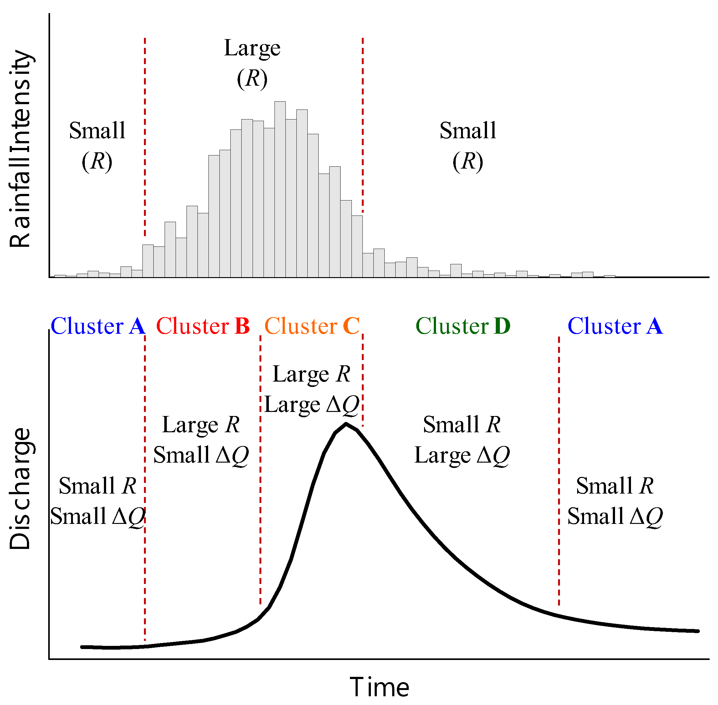
The rainfall-runoff process can be divided into several temporal steps corresponding to respective hydrologic phenomena. This study grouped rainfall-runoff data into clusters to represent different components of the rainfall-runoff process. An example of a typical rainfall event is shown in Figure 1a. Such an event generally begins with low rainfall (R), followed by intense, heavy rainfall, and finally ends with sprinkling rainfall. A storm hydrograph recorded during a storm rainfall event is presented in Figure 1b. At the beginning of the event, the discharge (Q) rises slowly and the discharge increment (ΔQ) is small. As the high intensity rainfall continues, the discharge increases rapidly to the peak discharge during the rising limb of the hydrograph. In the major part of the rising limb, the discharge increment is large. After cessation of the intense rainfall, the discharge declines sharply, but the discharge increment remains large. In the lower part of the recession limb, the discharge decreases slowly to the base flow and the discharge increment is small.
On the basis of the typical rainfall-runoff event illustrated in Figure 1, the rainfall-runoff process can be divided into several steps, as shown in Figure 2. At the beginning of a rainfall event, the rainfall is generally low and does not significantly contribute to the runoff. The rainfall-runoff data during this step are low rainfall and small discharge increments, and the data are grouped as Cluster A. Next, the rainfall increases and becomes large; however, the initial losses and high infiltration losses during this period cause only a gradual increase in the discharge. The high rainfall and small discharge increment data during this period are grouped as Cluster B. Subsequently, the infiltration losses decrease and increasingly more surface runoff reaches the basin outlet. The discharge increases rapidly to the crest segment of the hydrograph. The high rainfall and large discharge increment data are grouped as Cluster C. When the rainfall diminishes and the discharge starts to decrease, the data with low rainfall and large discharge increment are grouped as Cluster D. Subsequently, the segment of a hydrograph with low rainfall and small discharge increment is similar to the initial part of the hydrograph, and the corresponding data are thus also grouped as Cluster A. Thus, the rainfall-runoff process can be described by the sequence through Clusters A, B, C, D, and A. For an actual storm hydrograph, the rainfall-runoff phenomenon can be more complex, and the translation and storage effects can be significant in large watersheds. However, the proposed four clusters represent the rainfall-runoff process for a typical storm hydrograph.
2.2. Hybrid Neural Network Model
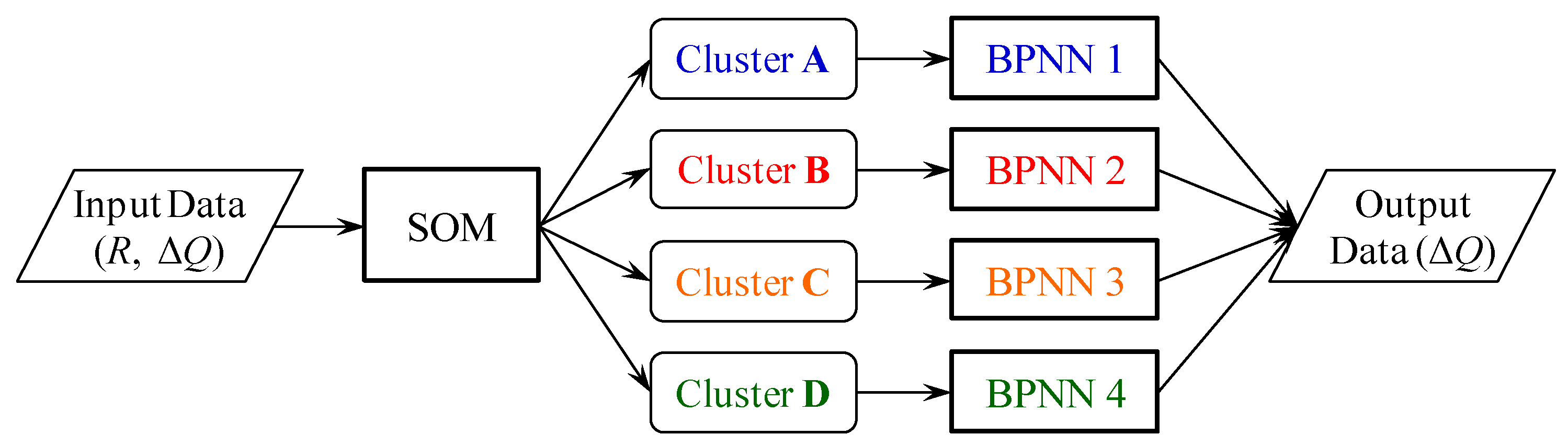
The proposed hybrid neural network model based on physically clustered hydrologic data is illustrated in Figure 3. The input rainfall and discharge increment data are grouped into four clusters using the SOM. Each cluster meaningfully corresponds to a typical step in the rainfall-runoff process. Then, BPNNs are constructed with respect to each cluster to forecast the discharge increment. The discharge forecasts are obtained when the forecasted discharge increment is added to the observed discharge at the present time. The detailed methodology of the SOM and BPNN has been well documented in the literature. Therefore, a brief description of the two neural network models is provided herein.
2.2.1. SOM
The SOM, proposed by Kohonen [34], is an unsupervised-learning neural network that automatically groups input data into several clusters without assigning the target outputs. The SOM uses a competitive learning strategy to map the input data onto a low-dimensional topological map. The process of constructing an SOM neural network is described briefly as follows.
The SOM network comprises one input layer and one output layer (the topological map), and the input neurons are fully connected to the output neurons. Let the input variables xi (i = 1, 2, …, m) form an input vector X, where m is the number of input neurons. Each output neuron uj (j = 1, 2, …, n) on the topological map has a weight wij with respect to each input variable xi, and n is the number of output neurons. The SOM is trained iteratively using randomly assigned initial weights. The SOM algorithm calculates the similarity between the input vector X and weight vector Wj for each output neuron. The similarity is defined as the Euclidean distance dj:
The output neuron whose weight vector is closest to the input vector has the minimum distance and is declared the winning neuron. The weights of this winning neuron and its neighboring neurons uj are then adjusted to approach the input vector. A typical neighborhood function is the Gaussian function hj:
where σ is the width of the topological neighborhood. The neighborhood function hj and width σ are usually set to decrease monotonically during the iterative process. The adjusted weight at iteration time r + 1 is defined as
where η is the learning rate (0 < η < 1) and is also set to decrease during the iterative process. Iterations are performed until the weight vector converges. Thereafter, similar input vectors are mapped to a specific region (cluster) on the topological map, and several clusters are automatically grouped.
2.2.2. BPNN
The BPNN, developed by Rumelhart et al. [35], is the most representative and popularly used neural network. A supervised multilayer feed-forward neural network, the BPNN uses the back-propagation algorithm for network training. The BPNN typically comprises three layers: the input, hidden, and output layers. Let the input variables xi (i = 1, 2, …, m) be the neurons in the input layer, and (k = 1, 2, …, p) be the output variable of the k-th neuron in the output layer. The BPNN output is expected to fit the target (actual) output yk. The BPNN (with n neurons in the hidden layer) can be expressed in the following form:
where wij is the weight connecting the i-th neuron in the input layer to the j-th neuron in the hidden layer; bj is the bias of the j-th hidden neuron; wjk is the weight connecting the j-th neuron in the hidden layer to the k-th neuron in the output layer; ck is the bias of the k-th output neuron; and F( ) is the activation function of the hidden neuron. Among the various activation functions that exist, linear, sigmoid, and hyperbolic tangent functions are the most widely used functions.
In the learning process of the back-propagation algorithm, the weights of the network are adjusted to minimize the objective function E:
3. Study Area and Hydrologic Data
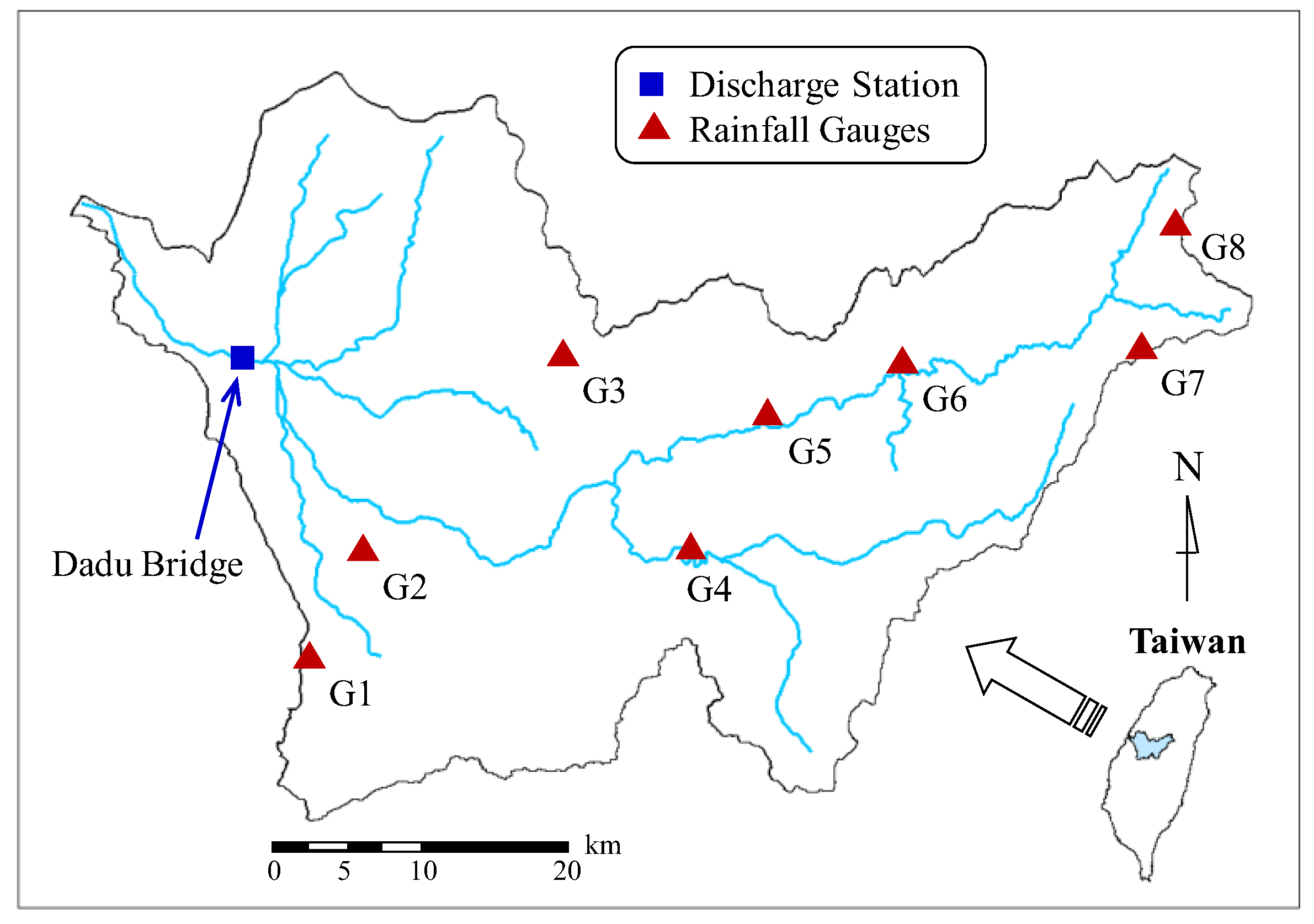
The study area is Wu River, located in central Taiwan (Figure 4). Wu River flows through the metropolitan area of Taichung City and empties into the Taiwan Strait. Wu River encloses a basin area of 2026 km2 and has a mainstream length of 119 km. The average annual precipitation in the Wu River basin is approximately 2087 mm, much of which is typhoon rainfall.
The downstream Dadu Bridge discharge station (Figure 4) near the metropolitan area is the forecasting object. This study collected hourly discharge data from Dadu Bridge and hourly rainfall data from eight rainfall gauges (named G1 to G8 and shown in Figure 4). Data for thirteen typhoon flood events with complete records were obtained. Among these flood events, 10 events (488 datasets) were used for calibration and three events (206 datasets) that caused flooding disasters in the downstream metropolitan area were used for validation. Table 1 lists the characteristics of the typhoon flood events, including the date and name of the typhoon, total amount of average rainfall (Thiessen polygon method) in the Dadu Bridge Basin, and peak discharge at Dadu Bridge.
4. Model Development and Forecasting Results
4.1. Determining the Input Variables
This study analyzed the lags between the discharge at Dadu Bridge with various lagged rainfall and discharge variables. The derived lagged variables were used as inputs of the proposed hybrid neural network model to forecast the discharge at Dadu Bridge. This study applied the linear transfer function (LTF) to determine the lagged variables by applying the least-squares technique to construct a linear function with lagged input variables. The t-test was employed to examine the statistical significance of the input variables. An advantage of using the LTF is that the lagged variables can be objectively determined by the statistical significance test. The process of using the LTF and the statistical significance test to determine the lags of input variables can be found in Chen et al. [38]. The time step for the analysis of lags and the following flood forecasting is one hour in this study.
This study used two types of hourly rainfall data as input variables: multiple rainfall data from eight rain gauges and average rainfall data. The most significant lags between the discharge at Dadu Bridge and the rainfall from each rain gauge were determined by the LTF. The lag for rain gauges G1 and G2 was 1 h, and the lag for G3 was 2 h. Rain gauges G4, G5, and G6 exhibited a lag of 3 h, and G7 and G8 exhibited a lag of 4 h. The determined lags were hydrologically rational. When the distance of a rain gauge to Dadu Bridge was longer, the most statistically significant time lag was also longer. For the average rainfall, the Thiessen polygon method was used to calculate the average rainfall in the Dadu Bridge watershed. The lagged average rainfall variables for 1–4 h were statistically significant at the 5% significance level, with the most significantly lagged variable for 3 h. The lagged discharge variables (discharge increment) were also examined. Only the lagged discharge variable for 1 h was statistically significant at the 5% significance level.
Let the hourly discharge of Dadu Bridge at the present time t be Q(t). For flood forecasting, the forecasted discharge with the lead-time of 1 h is . When the multiple rainfall data from eight rain gauges are used as inputs according to the most significant lags, the input variables are denoted as RG1(t), RG2(t), RG3(t − 1), RG4(t − 2), RG5(t − 2), RG6(t − 2), RG7(t − 3), and RG8(t − 3), where RG1(t) indicates the rainfall variable for rain gauge G1 at time t; the same notation applies to the other rain gauges. Let the discharge increment be ΔQ(t), which is defined as ΔQ(t) = Q(t) − Q(t − 1). The proposed hybrid neural network model using multiple rainfall data (denoted as fI[ ]) for forecasting the one-hour-ahead discharge increment can be formulated as
When the discharge increment is computed by the model and added to the observed discharge Q(t), the one-hour-ahead discharge can be forecasted. The model that uses the basin average rainfall data RA(t) (denoted as fII[ ]) is formulated as
For convenience, the hybrid neural network model using multiple rainfall data is hereafter termed Model I, and that using average rainfall data is termed Model II.
4.2. Clustering by Using the SOM
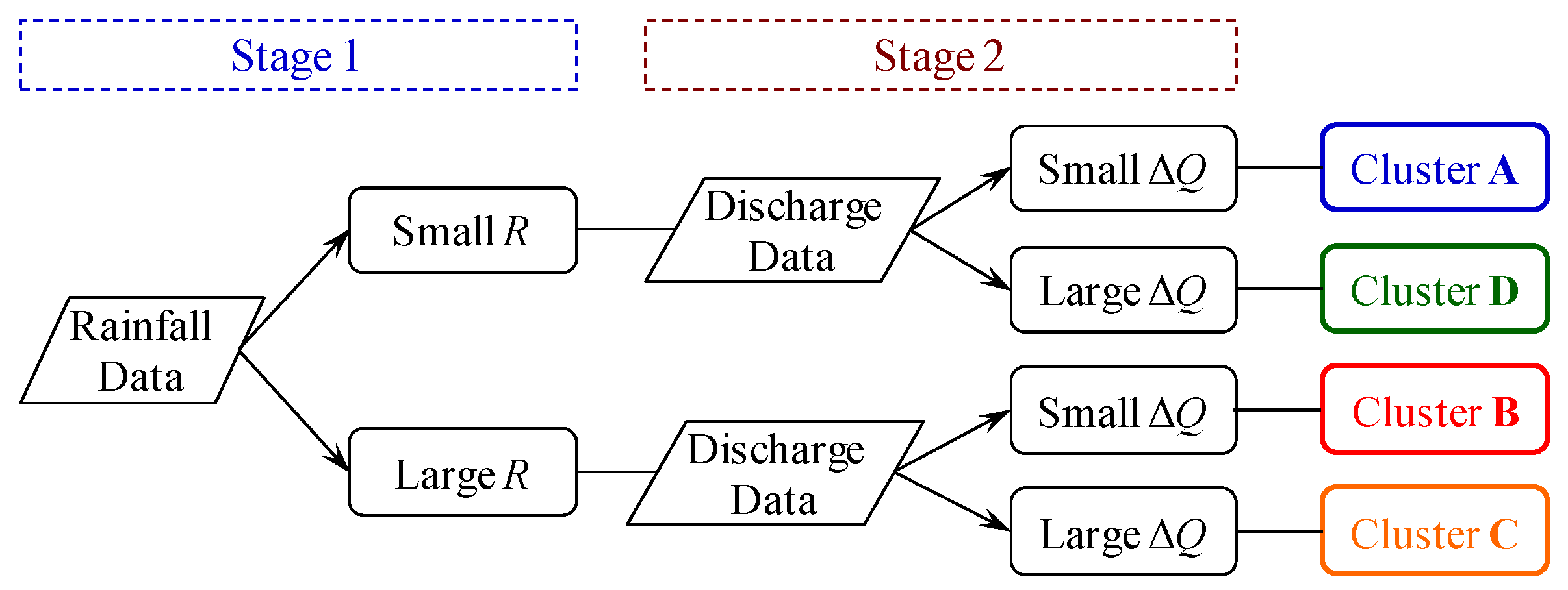
According to the proposed hybrid neural network model, input data were grouped into four hydrologically meaningful clusters formed by using the SOM. A two-stage clustering process (Figure 5) was proposed based on the properties of the rainfall and discharge data. In the first stage, input variables were grouped into two clusters (low and high rainfall clusters) by using only the rainfall data. In the second stage, the low rainfall cluster was further separated into two clusters (small and large discharge increment clusters) by using the discharge increment data. The high rainfall cluster was also divided into small and large discharge increment clusters. Consequently, four hydrologically meaningful clusters (with low and high R vs. small and large ΔQ) were obtained. This study applied the two-stage scheme to ensure that the rainfall and discharge increment data could be grouped into the expected four clusters. Because two forecasting models, Model I and Model II, were proposed corresponding to the two types of input rainfall variables, the clustering process was performed with respect to both the multiple rainfall data and average rainfall data.
Table 2 lists the clustering results for the calibration events (totally 488 datasets). The numbers of clusters corresponding to the two types of rainfall data are comparable. Cluster A (low R and small ΔQ) has the most data, and Cluster C (high R and large ΔQ) has the fewest data. The clustering results corresponding to the number of clusters are rational. The initial and final parts of the hydrograph (grouped as Cluster A) normally contain a large portion of the whole dataset. The rapidly rising limb of the hydrograph (grouped as Cluster C) encloses fewer data.
Table 3 lists the ranges (minimum and maximum) of rainfall R and discharge increment ΔQ for different clusters with respect to the average rainfall data. The average rainfall ≦4.66 mm was grouped into the low rainfall cluster, and that ≧4.67 mm was grouped into the high rainfall cluster at the first clustering stage. During the second-stage clustering process, the discharge increment data were further classified, and four clusters were obtained. The ranges of clusters are comparable to the physical meaning of clusters. According to the ranges listed in Table 3, Cluster A (low R and small ΔQ) has small rainfall and discharge increment data, and Cluster C (high R and large ΔQ) encloses the largest range among the clusters.
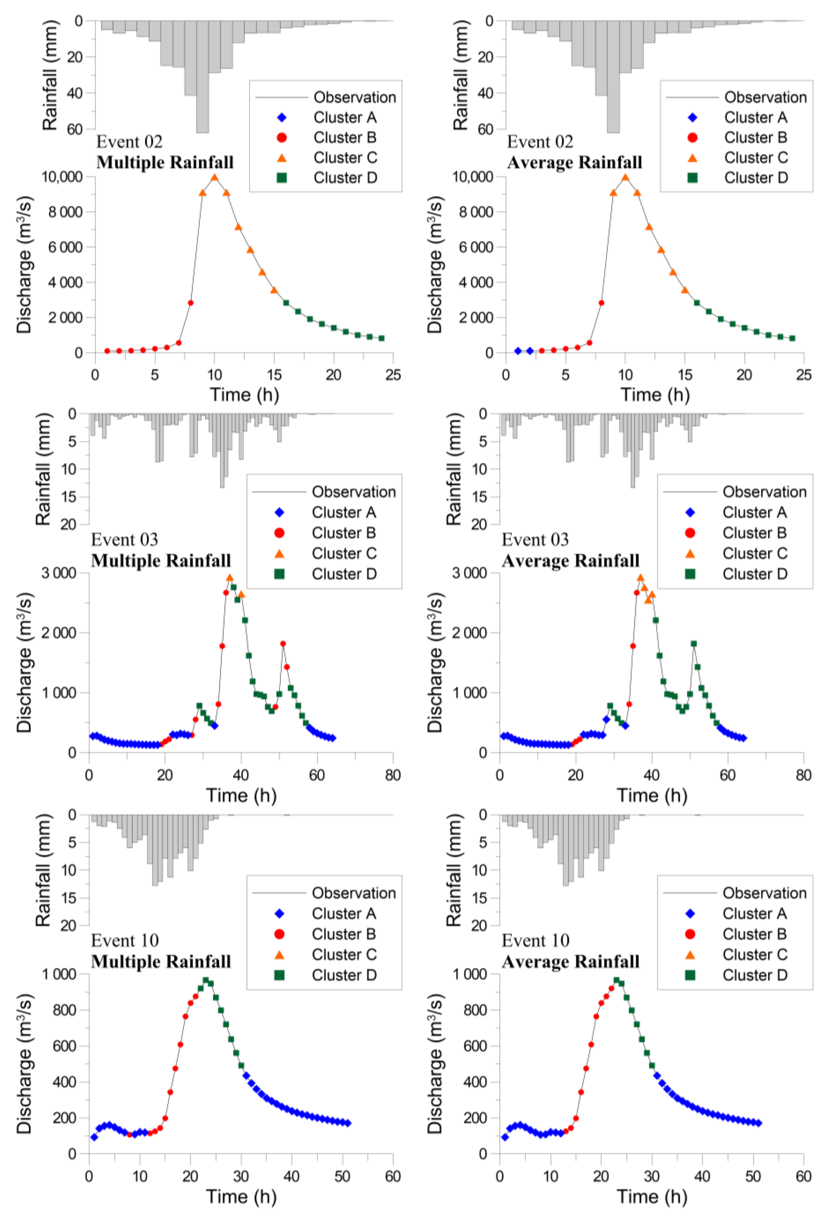
Figure 6 illustrates the clustering results of the SOM for the calibration events using three large, medium, and small flood events as an example. The clustering results concerning the multiple rainfall data (left panel) and average rainfall data (right panel) are similar. Event 02 (upper panel) is a large flood with a single peak caused by a concentrated and severe storm. The rainfall and discharge (also the discharge increment) data are large. Therefore, very few data (only two for the average rainfall case) are grouped as Cluster A. However, the rainfall-runoff process from Cluster B to Clusters C and D is appropriately identified by the clustered data. Event 03 (middle panel) is a medium flood with multiple peaks caused by a series of intermittent storms. The hydrologic process shown by the clusters is somewhat complicated. Nevertheless, progress from Cluster A to Clusters B, C, and D can be observed, with some data of Cluster C in the peak segment. Event 10 (lower panel) is an event with small peak discharge and low rainfall. The hydrograph is favorably described by the clusters; however, no data is grouped as Cluster C due to the low rainfall and discharge.
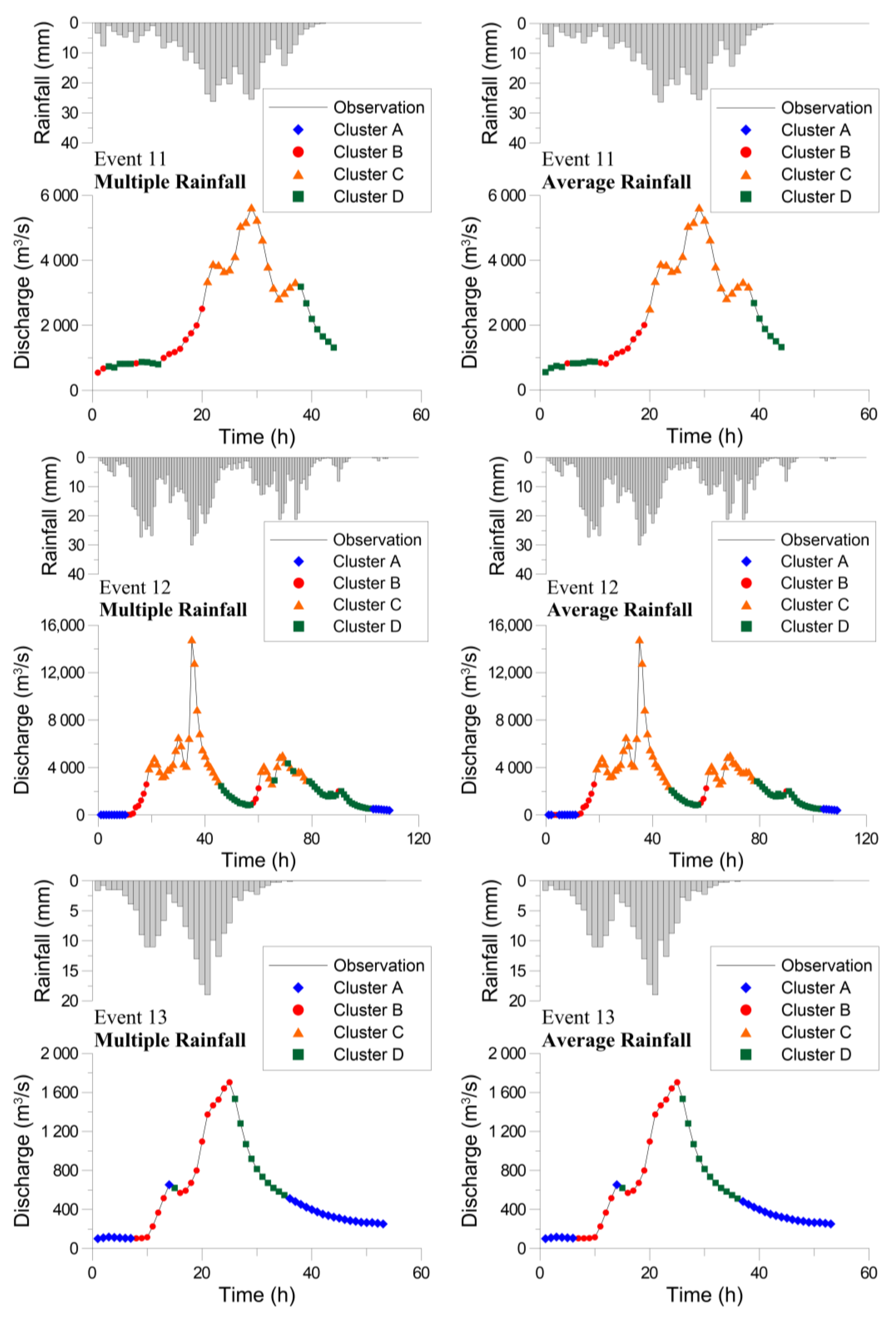
The SOM clustering was validated using the validation events, and the results are as follows. Two of the three events that caused flooding disasters in the metropolitan area were relatively large flood events. The greater numbers of Clusters C and D (with large discharge increments) than those of Clusters A and B (with small discharge increments) listed in Table 4 indicate the circumstances. Figure 7 presents the clustering results for the validation events. Event 11 is a large flood, with lots of data around the peak grouped as Cluster C and no data grouped as Cluster A. Event 12 is an extremely large flood with a peak discharge much higher than is present in the calibration data (cf. Table 1). Many high discharge data were reasonably classified as Cluster C. The clustering results show a clear progression from Cluster A to Clusters B, C, and D for the first hydrograph, and also an obvious sequence of Clusters B, C, D, and A for the second hydrograph. Event 13 is a small flood event that shows a similar result as Event 10 in the calibration set. The hydrograph is well explained by the clusters; however, no data is grouped as Cluster C. The calibration and validation results prove that the proposed clustering method based on the hydrologic process meaningfully depicts the physical processes behind rainfall and discharge data.
4.3. Flood Forecasting Using the Hybrid Neural Network Model
For each cluster, BPNNs were constructed with respect to the structures of Model I and Model II. The calibration data used in constructing the BPNNs were linearly normalized to the interval between 0 and 1 according to the minimum and maximum values in the calibration data. The hidden nodes and activation functions of the BPNNs were determined through trial and error. Table 5 lists the calibration results regarding the number of hidden nodes and types of activation functions. The numbers of hidden nodes of the BPNNs using multiple rainfall data are generally greater than those of the BPNNs using average rainfall data. The multiple rainfall data possess a more complex spatial pattern than the average rainfall data. Therefore, more hidden nodes are required to describe the complex relationship between the inputs and output. An interesting result is the derived activation functions. The BPNNs corresponding to Cluster A (small R and small ΔQ) and Cluster C (large R and large ΔQ) use the linear function. The BPNNs for Cluster B (large R and small ΔQ) and Cluster D (small R and large ΔQ) use the sigmoid function. When the rainfall and discharge increment data in a cluster have similar properties (i.e., all small or all large), the linear function is sufficient to model the input–output relationship. When the data in a cluster are different (i.e., small vs. large), the nonlinear sigmoid function is used to model the complex input–output relationship.
With the constructed SOMs and BPNNs, the hybrid neural network model was established for flood forecasting with respect to the calibration and validation events. Performance indices—the coefficient of efficiency (CE), mean absolute error (MAE), and error of time to peak discharge (ETP)—were obtained as follows:
where Q(t) is the observed discharge at time t; is the forecasted discharge; is the average observed discharge; n is the number of data; is the time to peak for observed discharge; and is the time to peak for forecasted discharge. CE is a dimensionless index with a value of unity indicating perfect fit. MAE is an index that directly describes the average forecast error with the same unit of the data. ETP is positive if the forecasted peak discharge is delayed. This lag often exists in hydrological forecasting. The model that has a smaller absolute value of ETP is better in forecasting performance.
Table 6 lists the performance indices of the hybrid neural network model for the calibration and validation events. The CE values for the calibration data are 0.97 and 0.98 corresponding to Model I and Model II, respectively, whereas the MAE values are 92.9 and 68.2 m3/s, which are small compared to the discharge magnitude of the flood events. For the validation events, CE is 0.94 and 0.91 and MAE is 188.0 and 248.2 m3/s, respectively. ETPs for calibration events range from −2 to 1 h; ETP is zero for half of the events. The average ETPs are small as shown in Table 6. The performance indices prove that the proposed hybrid neural network model favorably forecasts the flood discharge and that the performance of Model I and Model II is similar.
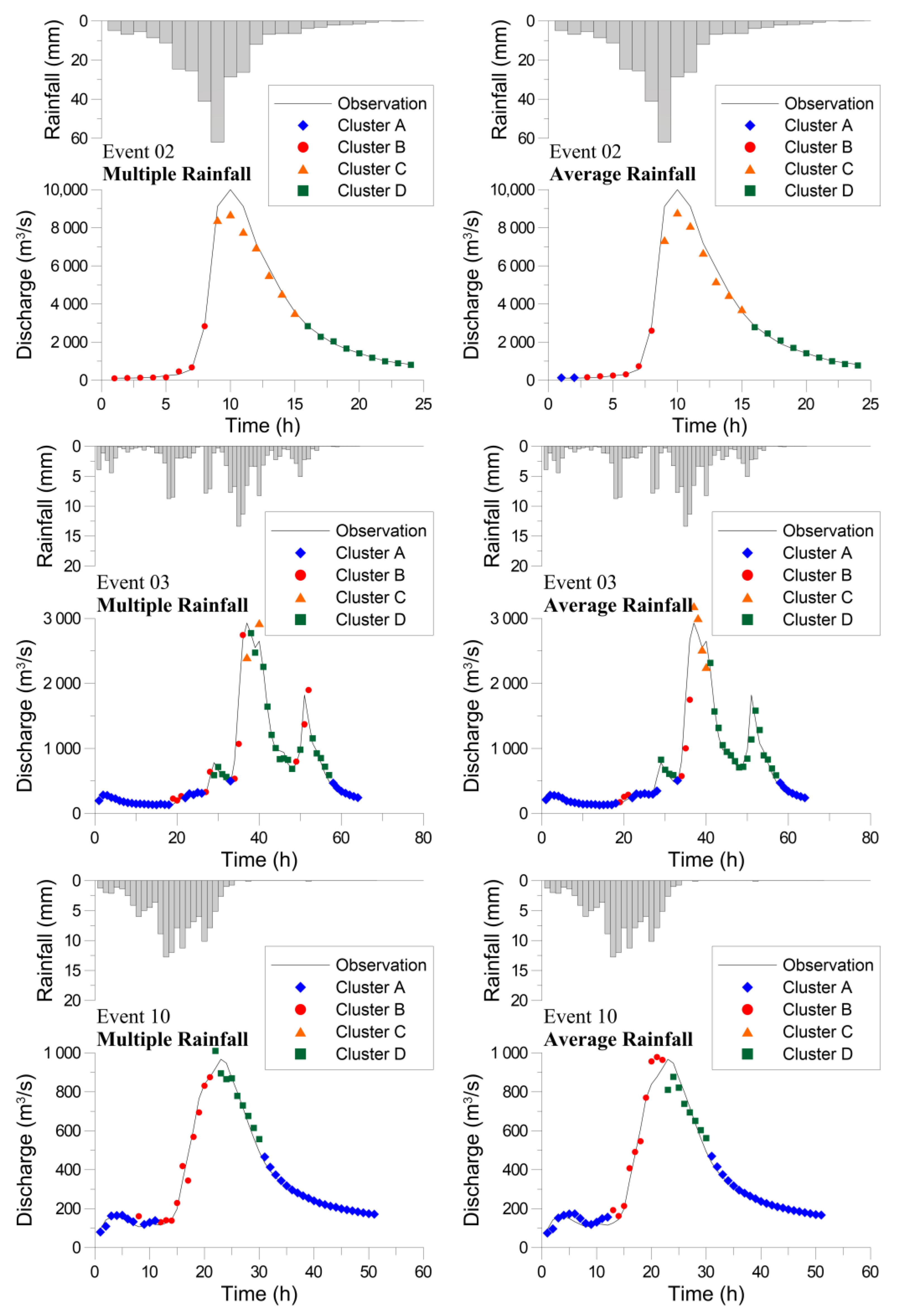
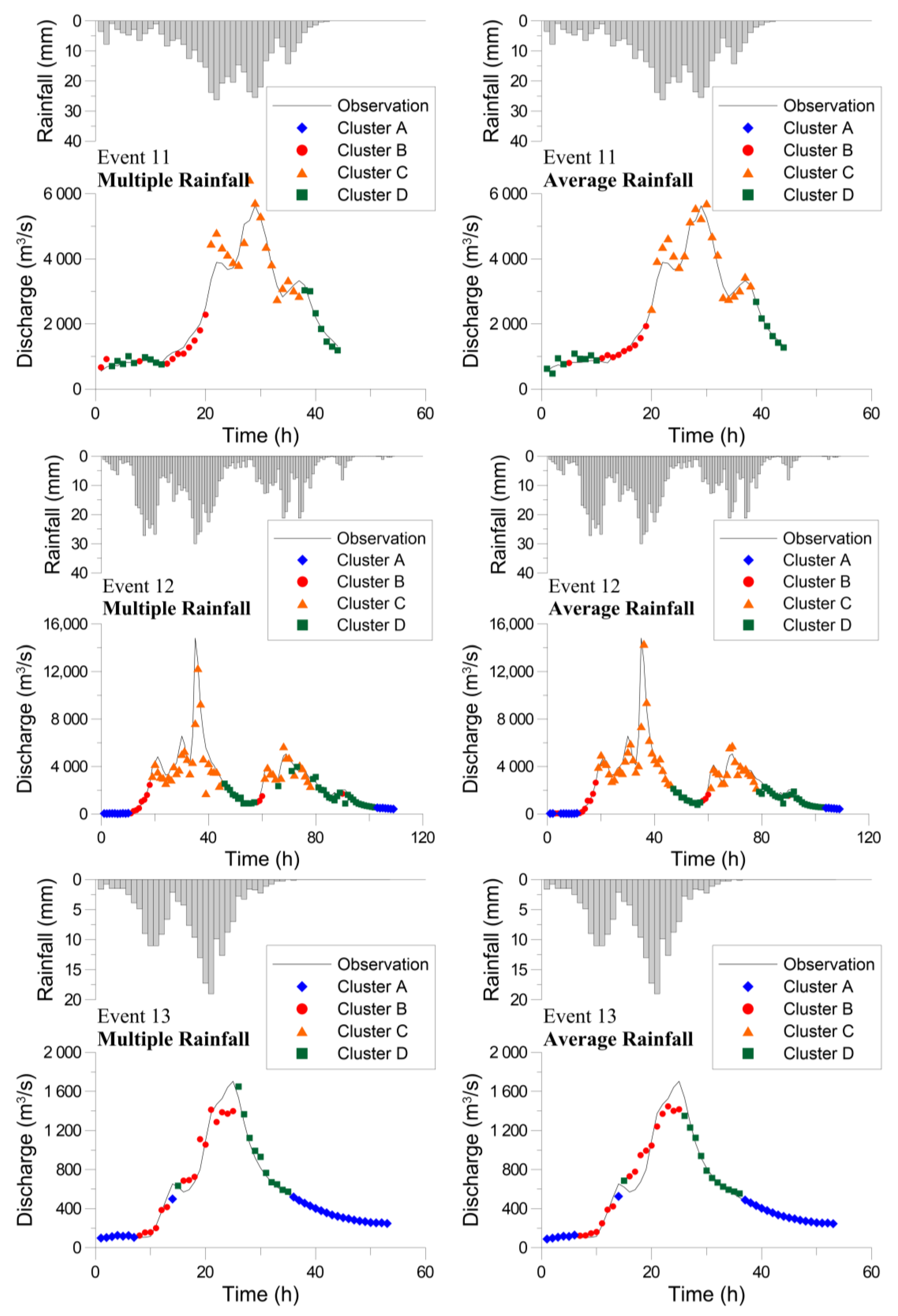
Figure 8 and Figure 9 present the forecasted hydrographs for the calibration and validation events, respectively. In general, the forecasted hydrograph matches the observed hydrograph. However, the forecasted discharge for Cluster C is not as close as that for the other clusters. During the model learning process, only 33 and 35 datasets were used to train the BPNNs for Cluster C (Table 2). Although the BPNNs trained using fewer data have larger errors, Event 12 has a peak discharge much higher than the calibration data. The forecasted discharges around the crest segment are reasonable, indicating that the hybrid neural network model extrapolates successfully. Overall, the forecasting results demonstrate that the proposed hybrid neural network model accurately forecasts typhoon floods, including small, medium, and large events, and the two types of model (Model I and Model II) have comparable capability.
4.4. Comparison with Traditional Neural Network Model
This study also developed a traditional neural network model to assess and compare its performance with that of the hybrid neural network model. The traditional neural network model, which does not group data into clusters, uses all the calibration data to construct a single BPNN using the same calibration scheme as the hybrid neural network model. The single BPNN was also trained by using the two types of rainfall variable (Model I and Model II). The constructed traditional BPNNs have three hidden nodes that use the sigmoid activation function. Table 7 lists the performance indices of the traditional neural network model. The CE value for calibration is 0.95, which is a little lower than the CE values (0.97 and 0.98) of the hybrid neural network model. However, the CE value of 0.85 for validation is considerably lower than those (0.94 and 0.91) of the hybrid neural network model. The MAE and the ETP values of the traditional BPNN are larger than those of the hybrid neural network model (cf. Table 6 and Table 7). Although the traditional BPNN also exhibits good forecasting performance in view of the performance indices, the hybrid neural network model apparently outperform the traditional neural network model.
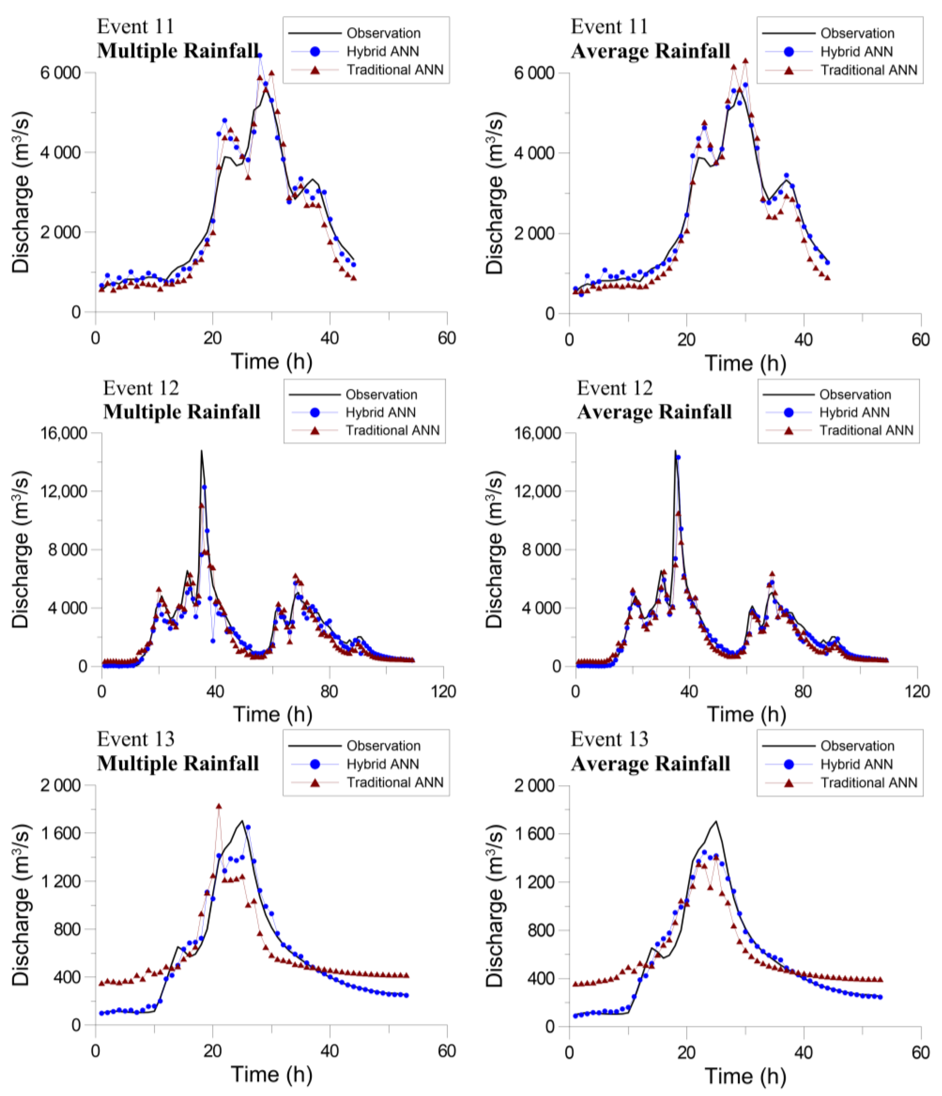
Figure 10 displays the forecasted hydrographs obtained using the hybrid and traditional neural network models pertaining to the validation events. In general, the two sets of the forecasted hydrographs have similar patterns. However, the hydrographs obtained using the traditional BPNN exhibit minor underestimation for large discharges (especially for the peak discharge in Event 12) and overestimation for small discharges (especially for the case in Event 13). The traditional BPNN was trained using small and large discharge data simultaneously. The learning mechanism matches the whole calibration data. Thus, the single BPNN does not perform very well in some cases of small and large discharges. However, the proposed hybrid neural network model was trained using different clusters with respective small and large datasets. The hybrid neural network model is more robust and flexible for various rainfall-runoff processes.
5. Conclusions
ANNs, usually regarded as black boxes, suffer from a lack of physical interpretation of the constructed model architecture. This study proposed a physical hybrid neural network model that combines the SOM and BPNNs and applied this proposed model to real-time flood forecasting. The SOM was used to group the rainfall and discharge data into four clusters with clear physical meanings to characterize the rainfall-runoff process. Then, a BPNN was constructed for each cluster with specific properties of rainfall and discharge data, which gave the BPNNs higher capability and a network structure that could be meaningfully discussed.
Typhoon flood discharges at Dadu Bridge and rainfall from eight rain gauges in the Wu River basin in Taiwan were used as the study data. Two types of rainfall data (multiple rainfall and average rainfall) were used to construct two types of hybrid neural network model (Model I and Model II). The lagged input variables of the models were determined by using the LTF. The derived lags of the rainfall variables are hydrologically rational and represent the distance from the rain gauge to the basin outlet.
The clustering results of the SOM pertaining to calibration and validation events prove that the hydrologic process is meaningfully described by the clusters. The rainfall-runoff process can be identified by the sequence of Clusters A, B, C, D, and A. The training of the BPNNs reveals that more hidden nodes are required to describe the complex relationship between multiple rainfall and discharge. The simple linear activation function was adopted in the clusters with similar data, whereas the nonlinear sigmoid activation function was used in clusters where the rainfall and discharge data were different.
Flood forecasting using the hybrid neural network model revealed that the proposed model successfully forecasts flood discharge with high efficiency and small errors. Both Model I and Model II have comparable forecasting performance. This study also developed a traditional neural network for comparison with the hybrid neural network model. The traditional neural network model that was trained with the whole calibration dataset did not perform favorably in some cases of small and large discharges. With respect to the performance indices and forecast hydrographs, the proposed physical hybrid neural network model exhibits robust flood forecasting and outperforms the traditional neural network model.
Author Contributions
Y.-D. Jhong and C.-S. Chen designed the research; H.-P. Lin and Y.-D. Jhong conducted the analysis; C.-S. Chen and S.-T. Chen supervised the study; Y.-D. Jhong and S.-T. Chen wrote the manuscript. All authors read and approved the final manuscript.
Conflicts of Interest
The authors declare no conflict of interest.
References
- Chang, F.J.; Chiang, Y.M.; Chang, L.C. Multi-step-ahead neural networks for flood forecasting. Hydrol. Sci. J. 2007, 52, 114–130. [Google Scholar] [CrossRef]
- Dawson, C.W.; Wilby, R. An artificial neural network approach to rainfall-runoff modelling. Hydrol. Sci. J. 1998, 43, 47–66. [Google Scholar] [CrossRef]
- French, M.N.; Krajewski, W.F.; Cuykendall, R.R. Rainfall forecasting in space and time using a neural network. J. Hydrol. 1992, 137, 1–31. [Google Scholar] [CrossRef]
- Lin, G.F.; Wu, M.C. A hybrid neural network model for typhoon-rainfall forecasting. J. Hydrol. 2009, 375, 450–458. [Google Scholar] [CrossRef]
- Lin, G.F.; Jhong, B.C.; Chang, C.C. Development of an effective data-driven model for hourly typhoon rainfall forecasting. J. Hydrol. 2013, 495, 52–63. [Google Scholar] [CrossRef]
- See, L.; Openshaw, S. Applying soft computing approaches to river level forecasting. Hydrol. Sci. J. 1999, 44, 763–778. [Google Scholar] [CrossRef]
- Young, C.C.; Liu, W.C. Prediction and modelling of rainfall-runoff during typhoon events using a physically-based and artificial neural network hybrid model. Hydrol. Sci. J. 2015, 60, 2102–2116. [Google Scholar] [CrossRef]
- Chen, S.T.; Yu, P.S.; Liu, B.W. Comparison of neural network architectures and inputs for radar rainfall adjustment for typhoon events. J. Hydrol. 2011, 405, 150–160. [Google Scholar] [CrossRef]
- Bray, M.; Han, D. Identification of support vector machines for runoff modeling. J. Hydroinf. 2004, 6, 265–280. [Google Scholar]
- Chen, S.T. Multiclass support vector classification to estimate typhoon rainfall distribution. Disaster Adv. 2013, 6, 110–121. [Google Scholar]
- Chen, S.T.; Yu, P.S. Real-time probabilistic forecasting of flood stages. J. Hydrol. 2007, 340, 63–77. [Google Scholar] [CrossRef]
- Chen, S.T.; Yu, P.S. Pruning of support vector networks on flood forecasting. J. Hydrol. 2007, 347, 67–78. [Google Scholar] [CrossRef]
- Han, D.; Chan, L.; Zhu, N. Flood forecasting using support vector machines. J. Hydroinf. 2007, 9, 267–276. [Google Scholar] [CrossRef]
- Lin, G.F.; Chen, G.R.; Huang, P.Y.; Chou, Y.C. Support vector machine-based models for hourly reservoir inflow forecasting during typhoon-warning periods. J. Hydrol. 2009, 372, 17–29. [Google Scholar] [CrossRef]
- Liong, S.Y.; Sivapragasam, C. Flood stage forecasting with support vector machines. J. Am. Water Resour. Assoc. 2002, 38, 173–186. [Google Scholar] [CrossRef]
- Yu, P.S.; Chen, S.T.; Chang, I.F. Support vector regression for real-time flood stage forecasting. J. Hydrol. 2006, 328, 704–716. [Google Scholar] [CrossRef]
- Yu, P.S.; Yang, T.C.; Chen, S.Y.; Kuo, C.M.; Tseng, H.W. Comparison of random forests and support vector machine for real-time radar-derived rainfall forecasting. J. Hydrol. 2017, 552, 92–104. [Google Scholar] [CrossRef]
- Ashrafi, M.; Chua, L.H.C.; Quek, C.; Qin, X. A fully-online Neuro-Fuzzy model for flow forecasting in basins with limited data. J. Hydrol. 2017, 545, 424–435. [Google Scholar] [CrossRef]
- Chang, F.J.; Chen, Y.C. A counterpropagation fuzzy-neural network modeling approach to real time streamflow prediction. J. Hydrol. 2001, 245, 153–164. [Google Scholar] [CrossRef]
- Lohani, A.K.; Kumar, R.; Singh, R.D. Hydrological time series modeling: A comparison between adaptive neuro-fuzzy, neural network and autoregressive techniques. J. Hydrol. 2012, 442, 23–35. [Google Scholar] [CrossRef]
- Mukerji, A.; Chatterjee, C.; Raghuwanshi, N.S. Flood forecasting using ANN, neuro-fuzzy, and neuro-GA models. J. Hydrol. Eng. 2009, 14, 647–652. [Google Scholar] [CrossRef]
- Nayak, P.C.; Sudheer, K.P.; Rangan, D.M.; Ramasastri, K.S. A neuro-fuzzy computing technique for modeling hydrological time series. J. Hydrol. 2004, 291, 52–66. [Google Scholar] [CrossRef]
- Nayak, P.C.; Sudheer, K.P.; Rangan, D.P.; Ramasastri, K.S. Short-term flood forecasting with a neurofuzzy model. Water Resour. Res. 2005, 41, W04004. [Google Scholar] [CrossRef]
- Nayak, P.C.; Sudheer, K.P.; Jain, S.K. Rainfall-runoff modeling through hybrid intelligent system. Water Resour. Res. 2007, 43, W07415. [Google Scholar] [CrossRef]
- Yarar, A. A hybrid wavelet and neuro-fuzzy model for forecasting the monthly streamflow data. Water Resour. Manag. 2014, 28, 553–565. [Google Scholar] [CrossRef]
- Zhang, G.; Patuwo, B.E.; Hu, M.Y. Forecasting with artificial neural networks: The state of the art. Int. J. Forecas. 1998, 14, 35–62. [Google Scholar] [CrossRef]
- Lange, N.T. New mathematical approaches in hydrological modeling–an application of artificial neural networks. Phys. Chem. Earth Part B 1999, 24, 31–35. [Google Scholar] [CrossRef]
- Jain, A.; Sudheer, K.P.; Srinivasulu, S. Identification of physical processes inherent in artificial neural network rainfall runoff models. Hydrol. Process. 2004, 18, 571–581. [Google Scholar] [CrossRef]
- Chen, S.T. Mining informative hydrologic data by using support vector machines and elucidating mined data according to information entropy. Entropy 2015, 17, 1023–1041. [Google Scholar] [CrossRef]
- Furundzic, D. Application example of neural networks for time series analysis: Rainfall–runoff modeling. Signal Process. 1998, 64, 383–396. [Google Scholar] [CrossRef]
- Abrahart, R.J.; See, L. Comparing neural network and autoregressive moving average techniques for the provision of continuous river flow forecasts in two contrasting catchments. Hydrol. Process. 2000, 14, 2157–2172. [Google Scholar] [CrossRef]
- Hsu, K.L.; Gupta, H.V.; Gao, X.; Sorooshian, S.; Imam, B. Self-organizing linear output map (SOLO): An artificial neural network suitable for hydrologic modeling and analysis. Water Resour. Res. 2002, 38, 38-1–38-17. [Google Scholar] [CrossRef]
- Jain, A.; Srinivasulu, S. Integrated approach to model decomposed flow hydrograph using artificial neural network and conceptual techniques. J. Hydrol. 2006, 317, 291–306. [Google Scholar] [CrossRef]
- Kohonen, T. Self-organized formation of topologically correct feature maps. Biol. Cybern. 1982, 43, 59–69. [Google Scholar] [CrossRef]
- Rumelhart, D.E.; Hinton, G.E.; Williams, R.J. Learning representations by back-propagating errors. Nature 1986, 323, 533–536. [Google Scholar] [CrossRef]
- Hagan, M.T.; Demuth, H.B.; Beale, M.H. Neural Network Design; PWS Publishing: Boston, MA, USA, 1996. [Google Scholar]
- Haykin, S. Neural Networks: A Comprehensive Foundation; MacMillan: New York, NY, USA, 1994. [Google Scholar]
- Chen, C.S.; Chen, B.P.T.; Chou, F.N.F.; Yang, C.C. Development and application of a decision group back-propagation neural network for flood forecasting. J. Hydrol. 2010, 385, 173–182. [Google Scholar] [CrossRef]
Figure 1.
Example of a typical rainfall and runoff event. (a) Rainfall hyetograph; (b) Flood hydrograph.
Figure 1.
Example of a typical rainfall and runoff event. (a) Rainfall hyetograph; (b) Flood hydrograph.

Figure 2.
Rainfall-runoff clusters based on the hydrologic process.

Figure 3.
Structure of the proposed hybrid neural network model.

Figure 4.
Wu River basin and locations of the gauge stations.

Figure 5.
Process of the two-stage clustering scheme.

Figure 6.
Clustering results of the self-organizing map (SOM) for three calibration events.

Figure 7.
Clustering results of the SOM for the validation events.

Figure 8.
Flood forecasting results of the proposed model for calibration events.

Figure 9.
Flood forecasting results of the proposed model for validation events.

Figure 10.
Comparison of the flood forecasting results for the hybrid and traditional neural network models.
Figure 10.
Comparison of the flood forecasting results for the hybrid and traditional neural network models.


Table 1.
Characteristics of collected typhoon flood events.
| Event No. | Date | Typhoon | Total Rainfall (mm) | Peak Discharge (m3/s) | Note |
|---|---|---|---|---|---|
| 01 | 4 August 1998 | Otto | 100.9 | 1440 | Calibration |
| 02 | 30 July 2001 | Toraji | 290.4 | 10,000 | Calibration |
| 03 | 16 September 2001 | Nari | 165.0 | 2930 | Calibration |
| 04 | 20 June 2012 | Talim | 95.5 | 1067 | Calibration |
| 05 | 1 August 2012 | Saola | 452.1 | 7199 | Calibration |
| 06 | 12 July 2013 | Soulik | 358.6 | 11,004 | Calibration |
| 07 | 21 August 2013 | Trami | 319.6 | 2011 | Calibration |
| 08 | 29 August 2013 | Kongrey | 127.0 | 1786 | Calibration |
| 09 | 7 August 2015 | Soudelor | 138.8 | 720 | Calibration |
| 10 | 28 September 2015 | Dujuan | 134.9 | 967 | Calibration |
| 11 | 31 July 1996 | Herb | 415.3 | 5630 | Validation |
| 12 | 1 July 2004 | Mindulle | 898.4 | 14,802 | Validation |
| 13 | 22 July 2014 | Matmo | 193.8 | 1704 | Validation |
Table 2.
Number of clusters for the calibration data sets.
| Cluster | Model I(Multiple Rainfall) | Model II(Average Rainfall) |
|---|---|---|
| Cluster A (Low R, Small ΔQ) | 222 | 231 |
| Cluster B (High R, Small ΔQ) | 98 | 89 |
| Cluster C (High R, Large ΔQ) | 33 | 35 |
| Cluster D (Low R, Large ΔQ) | 135 | 133 |
Table 3.
Ranges of rainfall and discharge increment for different clusters.
| Cluster | Rainfall (mm) | Discharge Increment (m3/s) | ||
|---|---|---|---|---|
| Min. | Max. | Min. | Max. | |
| Cluster A | 0 | 4.66 | −80 | 261 |
| Cluster B | 4.67 | 45.21 | −303 | 4756 |
| Cluster C | 4.84 | 51.83 | −3170 | 6280 |
| Cluster D | 0 | 4.56 | −750 | 841 |
Table 4.
Number of clusters for the validation datasets.
| Cluster | Model I(Multiple Rainfall) | Model II(Average Rainfall) |
|---|---|---|
| Cluster A (Low R, Small ΔQ) | 42 | 43 |
| Cluster B (High R, Small ΔQ) | 40 | 40 |
| Cluster C (High R, Large ΔQ) | 59 | 60 |
| Cluster D (Low R, Large ΔQ) | 65 | 62 |
Table 5.
Calibrated numbers of hidden nodes and types of activation functions.
| Cluster | Model I | Model II | ||
|---|---|---|---|---|
| Number of Hidden Nodes | Activation Function | Number of Hidden Nodes | Activation Function | |
| Cluster A (Low R, Small ΔQ) | 3 | Linear | 2 | Linear |
| Cluster B (High R, Small ΔQ) | 3 | Sigmoid | 2 | Sigmoid |
| Cluster C (High R, Large ΔQ) | 2 | Linear | 2 | Linear |
| Cluster D (Low R, Large ΔQ) | 4 | Sigmoid | 2 | Sigmoid |
Table 6.
Performance indices of the hybrid neural network model.
| Data | Model Type | CE | MAE (m3/s) | ETP (h) |
|---|---|---|---|---|
| Calibration | Model I | 0.97 | 92.9 | –0.2 |
| Model II | 0.98 | 68.2 | –0.1 | |
| Validation | Model I | 0.94 | 188.0 | 0.3 |
| Model II | 0.91 | 248.2 | 0.0 |
Table 7.
Performance indices of the traditional neural network model.
| Data | Model Type | CE | MAE (m3/s) | ETP (h) |
|---|---|---|---|---|
| Calibration | Model I | 0.95 | 229.2 | –0.1 |
| Model II | 0.95 | 242.4 | –0.5 | |
| Validation | Model I | 0.85 | 339.8 | –1.0 |
| Model II | 0.85 | 359.1 | 0.7 |
© 2018 by the authors. Licensee MDPI, Basel, Switzerland. This article is an open access article distributed under the terms and conditions of the Creative Commons Attribution (CC BY) license (http://creativecommons.org/licenses/by/4.0/).
Share and Cite
MDPI and ACS Style
Jhong, Y.-D.; Chen, C.-S.; Lin, H.-P.; Chen, S.-T. Physical Hybrid Neural Network Model to Forecast Typhoon Floods. Water 2018, 10, 632. https://doi.org/10.3390/w10050632
AMA Style
Jhong Y-D, Chen C-S, Lin H-P, Chen S-T. Physical Hybrid Neural Network Model to Forecast Typhoon Floods. Water. 2018; 10(5):632. https://doi.org/10.3390/w10050632
Chicago/Turabian StyleJhong, You-Da, Chang-Shian Chen, Hsin-Ping Lin, and Shien-Tsung Chen. 2018. "Physical Hybrid Neural Network Model to Forecast Typhoon Floods" Water 10, no. 5: 632. https://doi.org/10.3390/w10050632
Note that from the first issue of 2016, this journal uses article numbers instead of page numbers. See further details here.