Analyzing the Role of Shallow Groundwater Systems in the Water Use of Different Land-Use Types in Arid Irrigated Regions
by
 ,
,
Dongyang Ren
1,2, 
Xu Xu
1,2,*,
Quanzhong Huang
1,2,
Zailin Huo
2, 
Yunwu Xiong
1,2 and
Guanhua Huang
1,2 1
Chinese-Israeli International Center for Research and Training in Agriculture, China Agricultural University, Beijing 100083, China
2
Center for Agricultural Water Research, China Agricultural University, Beijing 100083, China
*
Author to whom correspondence should be addressed.
Water 2018, 10(5), 634; https://doi.org/10.3390/w10050634
Submission received: 5 March 2018
/
Revised: 18 April 2018
/
Accepted: 4 May 2018
/
Published: 15 May 2018
(This article belongs to the Section Water, Agriculture and Aquaculture)
Abstract
:Clarifying the role of shallow groundwater systems in eco-hydrological processes is of great significance to agricultural production and ecological sustainability. In this paper, a lumped water balance model was proposed for the GSPAC (groundwater-soil-plant-atmosphere-continuum) system for different land use types under arid, shallow water table conditions. Model application was conducted in an irrigation district (Jiyuan) located in the upper Yellow River basin. A 13-year (2001–2013) water balance calculation was carried out to quantify the water budgets of different land use types. The effects of shallow groundwater on water and salt exchanges among different land use patterns were analyzed. Results indicated the shallow groundwater systems played a significant role in water storage and supply, water and salt redistribution, and the salt accumulation and drainage in Jiyuan. About 36% of the total applied water was first stored in a shallow groundwater system, and then redistributed. After redistribution, 63% of the total diverted water was consumed by cropland evapotranspiration (ET), 20% by natural land ET; the rest was discharged through drainage or groundwater exploitation. Finally, 67% of the introduced salt accumulated in natural land, while the rest was drained away, which helped maintain the productivity of the croplands. Overall, our results have quantitatively revealed the multifaceted roles of shallow groundwater systems, and also suggested the key management concepts for sustaining agroecosystems in arid irrigated areas.
1. Introduction
Shallow water tables are a common feature of many irrigated agricultural systems [1], such as the irrigation districts along the Yellow River in China [2,3], the Fergana Valley in Central Asia [4], the inland valleys in West Africa [5], the irrigated areas in the arid western United States [6] and south-eastern Australia [7], and the Indo-Gangetic Plain in India and Pakistan [8]. In these areas, shallow groundwater is a key factor in eco-hydrological processes relating to evaporation, transpiration, soil water-salt dynamics, and ground water flow. It may have a positive (water supply) or negative (waterlogging or soil salinization) impact on crops and natural vegetation [9,10,11,12].
Thoroughly understanding the role of shallow groundwater systems in agro-hydrological processes is of great significance to water management, as well as the sustainability of agroecosystems. Evaluation of the role of shallow groundwater is feasible only when all groundwater flow terms are known. Saturated–unsaturated water flow models, such as HYDRUS [13] and SWAP [14], can give a detailed description of the interaction between shallow groundwater, soil and plant. However, these models are traditionally considered as field scale models, and seldom used in the regional scale. Many widely used groundwater models, such as MODFLOW [15] and FEFLOW [16], can simulate 3D groundwater flows on a regional scale, on the basis of locally measured hydrogeological properties and boundary conditions. However, they mainly focus on relatively deep groundwater systems, and the interaction between groundwater and the root zone is seldom considered. Due to the (reverse) Wieringermeer effect [17,18] and Lisse effect [19] in shallow water table regions [20], groundwater dynamics are very difficult to simulate. Numerical models are still not adequate for use in regional simulations of shallow water table areas.
The lumped water balance method has been widely used to predict streamflow, lake levels, groundwater recharge and exchange, and to plan irrigation schemes for crops [21,22,23]. Water balance equations are often used to determine the hydrologic components that are difficult to obtain, and are, superficially, the most convincing method. They have several advantages, like straightforward implementation, relatively low cost, and applicability to all types of groundwater conditions [24]. However, such equations can only be solved when no more than one term is unknown. Usually, both ET in the upper boundary, and the groundwater flow through lateral boundary, are unknown in practice. Therefore, the water balance method is more suitable for relatively closed basins at a given time scale (e.g., monthly). It is not easy to determine the detailed spatio-temporal pattern of water budgets. Nevertheless, by coupling it with some empirical equations, the water balance method could still be considered the most efficient method in large-scale and long-term water resource assessment and management.
The Hetao Irrigation District (Hetao) located in the upper Yellow River basin (Figure 1) is a representative area with shallow water tables [25]. Due to the arid to semi-arid continental climate, about 5 billion m3 of irrigation water is diverted from the Yellow River each year to Hetao, and basin irrigation is applied [26,27]. As a result, the depth to the water table is very shallow, especially during the irrigation period. The shallow groundwater has caused waterlogging and salinity problems in many parts of the region, but has also served as a water source for the natural vegetation, and provided a path way for irrigation water redistribution and reuse [28,29]. Due to water scarcity, water saving practices are being implemented both at farm and district levels, including lining canals, upgrading irrigation scheduling, adopting precise land leveling, and modern irrigation technologies [23,26,30]. With the application of water saving practices, the groundwater level is declining in many parts of Hetao, and the current balance of the shallow groundwater system may be interrupted. The declining water level may favor the control of waterlogging and salinity, but may also cause the degradation of natural vegetation, and increase drought risks. The question of whether there is a trade-off between the positive and negative effects of the shallow groundwater has not been fully examined.
Therefore, in this study, a lumped water balance model was developed for the GSPAC (groundwater-soil-plant-atmosphere-continuum) system for different land use types, and adopted to quantify the water budgets of an irrigation system located in the western of Hetao. A 13-year water balance calculation was carried out to analyze the water income and losses of different land use types. The objectives of this study were to assess the role of shallow groundwater systems in water use in arid irrigated agro-ecosystems, and to provide some new insights into irrigation management and groundwater control.
2. Materials and Methods
2.1. The Study Area
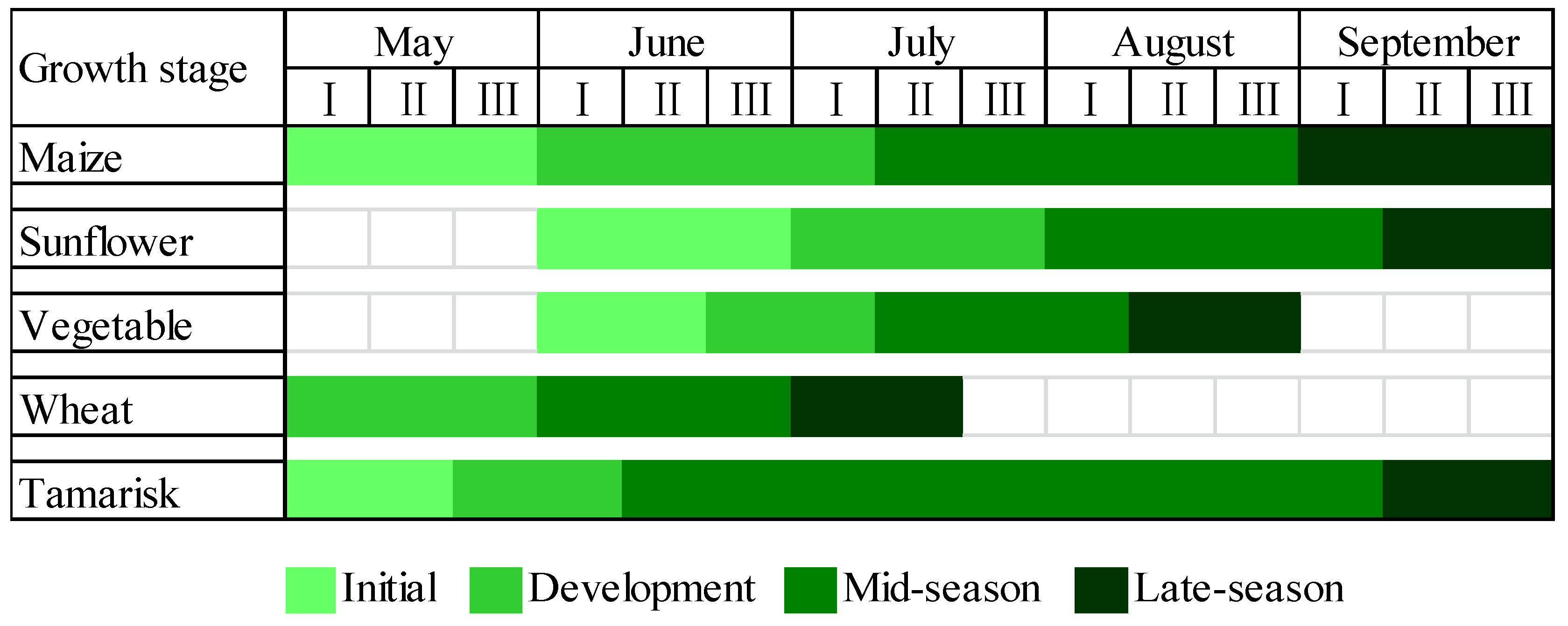
The Jiyuan Irrigation System (Jiyuan) (Figure 1) (40°45′–40°52′ N, 106°59′–107°07′ E), located in the western region of the Hetao, was selected as a typical case study region. The land use map of Jiyuan in this study was derived by manual visual interpretation of high-resolution Google Earth images (image date 4 September 2013, about 0.5 m resolution) (Figure 1). Results show that it covers an area of 8490 ha, in which 60.7% is cropland, 30.3% is natural land, 5.7% is residential land, 2.5% is sand dune, and 0.8% is water body. The croplands dominated the landscape in Jiyuan, with various kinds of crops, including sunflower, maize, wheat and some vegetables (e.g., watermelon, tomato and pepper). In recent years, sunflower and maize are the main crops grown in Jiyuan, occupying more than 80% of the croplands. The other land use types exhibit a patchy distribution within and surrounding the croplands. The natural lands are mainly sparse grassland with scattered shrubs or formerly cultivated land which had been abandoned because of high soil salinization. The species composition of natural vegetation is simple: mainly salt-tolerant vegetation, such as Tamarix chinensis, Phragmites australis and Elymus dahuricus. The growth stages of the main crops and natural vegetation are shown in Figure 2. Residential land consists of built-up areas for rural settlements. About 15,000 people inhabit the region. The sand dunes are located in the south and west of Jiyuan, and have very low plant cover (usually less than 10%). The water bodies here are mainly fishponds.
The area has an arid to semi-arid continental climate in which water resources are relatively scarce, with an average annual precipitation of 140 mm (Figure 3) and mean annual evaporation (20 cm pan) of approximately 2000 mm. Nearly 90% of the precipitation occurs during the growing season (May to September). The topography is very flat, with plain elevation declining from 1043 to 1036 m from the south to north. Besides the regional terrain trend, elevation differences exist among different land covers, e.g., natural lands are always 0.3–0.5 m lower than the nearby croplands, and sand dunes are usually about 2–3 m higher. The flat topography and poor drainage systems combined with significant irrigation determine the presence of shallow water tables (varies from 0 to 3 m) and the long-term accumulation of salts derived from irrigation water. The average groundwater hydraulic gradient is small (about 0.05%) at the regional scale, whereas on the landscape scale (30–500 m), groundwater hydraulic gradients can reach 1–3% among different land use types during the irrigation period, due to the uneven irrigation. Thus, the lateral groundwater exchange among different land uses is very significant.
Hetao is a closed rift basin underlain by Quaternary sediments (mainly lake sediments and alluvial deposits of the Yellow River). As a part of Hetao, the Jiyuan has an unconfined aquifer with a depth of 100–150 m. The deposits of the upper 6–25 m are mainly silt loam and sandy loam (USDA), with hydraulic conductivity of about 0.03–0.1 md−1, while the deposits below this layer are mainly sand and loamy sand with hydraulic conductivity of 4–18 md−1 [23].
For the shallow groundwater system, Jiyuan is a relatively closed basin with minimal connectivity to adjacent areas. Its north and east boundaries are the main drainage ditches which discharge water out of the region, while the south and west boundaries are a series of discontinuous ditches which drain and store excess water. One main drainage ditch in the middle Jiyuan flows from south to north, draining water to the north ditch. The irrigation network in Jiyuan is controlled by two branch canals (i.e., the west branch and the east branch) which originate from the same trunk canal, and flow from south to north (Figure 1). Besides these main canals and ditches, numerous lateral canals/ditches, tertiary canals/ditches and terminal canals/ditches constitute the irrigation and drainage system of Jiyuan.
2.2. Field Observations and Data Collection
Field observations were conducted in Jiyuan in 2012 and 2013. A total of 28 observation points and 39 observation wells were set at Jiyuan (Figure 1). Each of the observation points also contains an observation well. Soil sampling was performed monthly from the soil surface to the groundwater level, using a soil auger at each of the observation points. The soil samples were collected every 20 cm to obtain the layered soil moisture and salt contents. The groundwater level and groundwater electrical conductivity were observed every 5–15 days in the observation wells. Some typical wells were also recorded more frequently by water level loggers. Water diversion, field irrigation, and drainage were observed during the irrigation period. The range of irrigation depths to different crop fields during the growing season is shown in Table 1. Soils in the top 0–3 m are mainly silt loam. Meanwhile, some more detailed field observations on a smaller scale were conducted in the Yangchang canal command area (YCA) (Figure 1) within Jiyuan, as described in Ren et al. [28]. Based on the two-year field observations and former studies [31], the following results were obtained: a specific yield of 0.062; a canal conveyance efficiency (the ratio of water volume delivered to the fields to the water diverted into the canals) of 0.71; and a canal seepage ratio (the ratio of groundwater recharge from canal seepage to the water diverted into the canals) of 0.195.
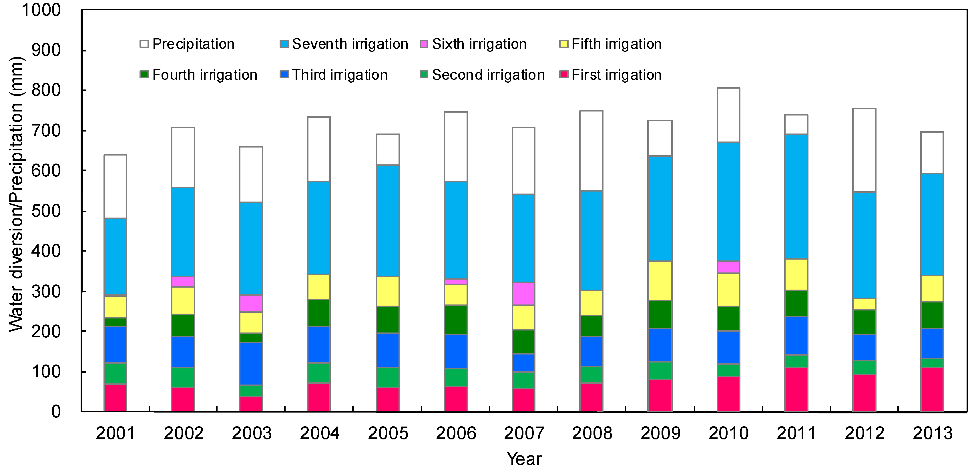
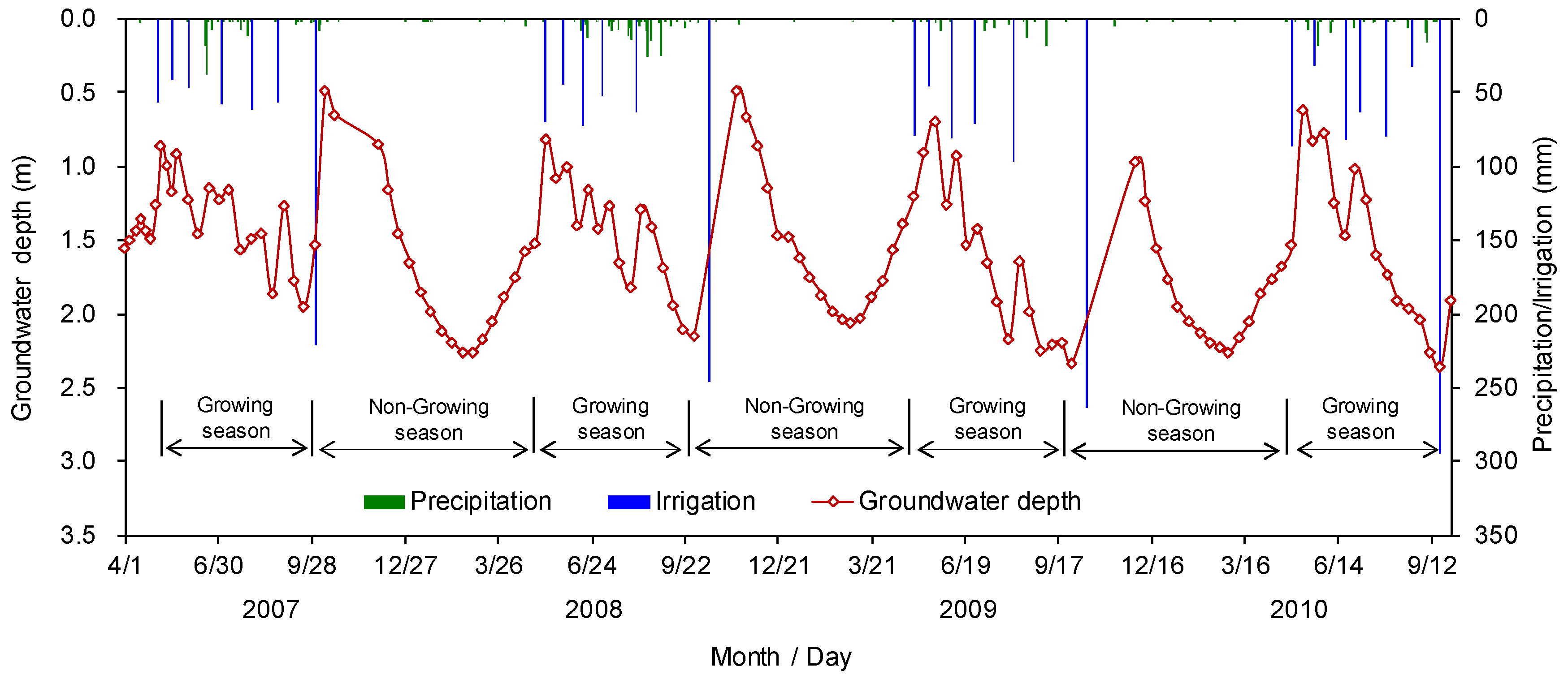
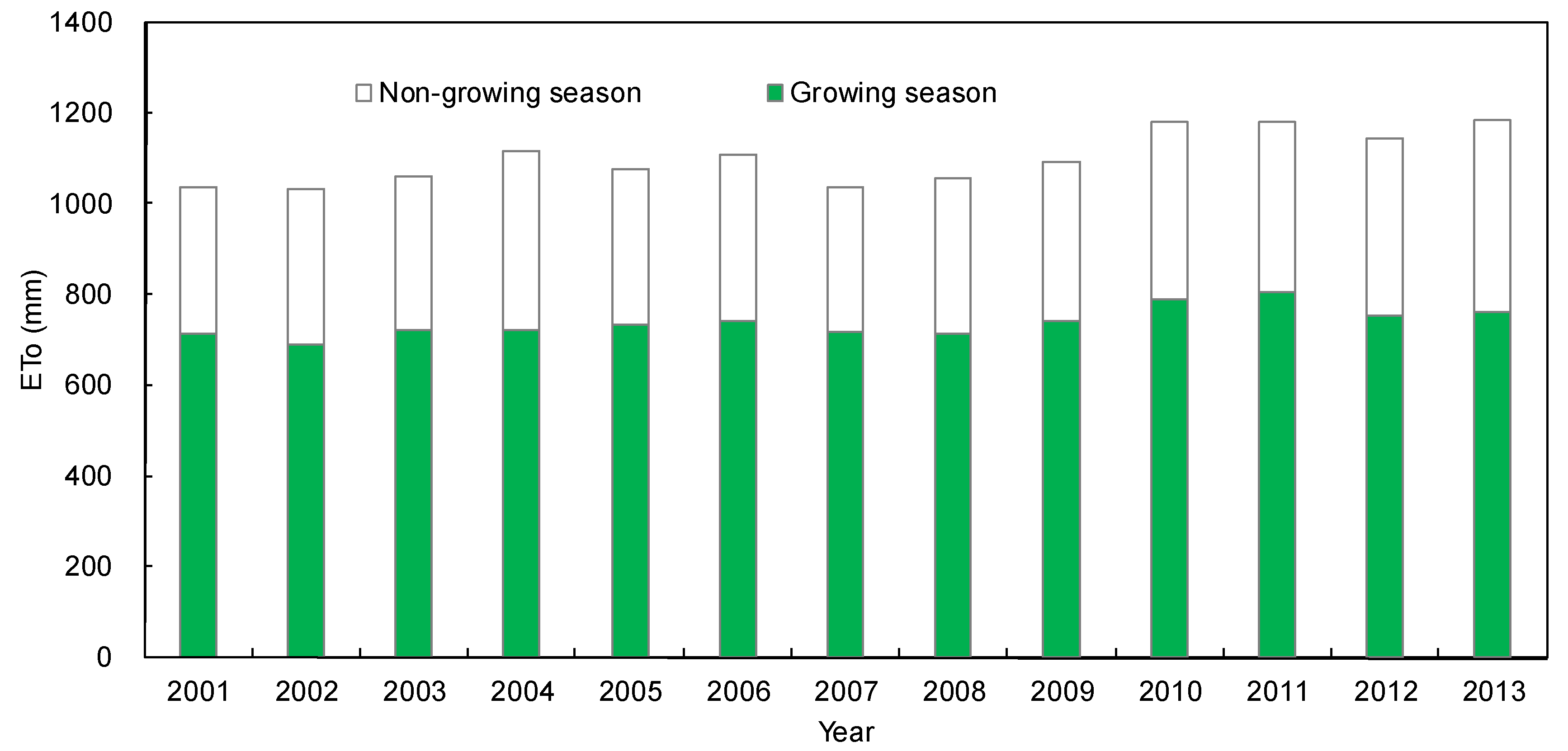
Information on water conveyance from 2001 to 2013 in the two branch canals was collected from the Hetao Irrigation District Administration. Generally, Jiyuan has seven water diversions throughout the year, with the first six occurring during the growing season, and the seventh (autumn irrigation) during the non-growing season (Figure 3). Total water diversion in Jiyuan averaged 49 million m3 (580 mm) in the period from 2001–2013, of which the autumn irrigation accounted for more than 40% (Hetao Irrigation District Administration, 2001–2013). The total amounts of water diversion are largely dependent on precipitation. In the dry years, water diversions were usually larger than in wet years, to alleviate water deficits (Figure 3). Drainage data was also collected from the local administration. Based on the statistical data, the drainage amount averaged 5.75 million m3 (68 mm) during the year, in which about 1/3 was through groundwater drainage; the rest was the return water (i.e., the excessive irrigation water directly released into the drainage ditches). Groundwater level data over a 5-day interval observed in three wells from 2001 to 2013, and observed in 50 wells from 2007 to 2010, were also collected from the Shahaoqu experimental station (Figure 4). Daily meteorological data, including precipitation, air temperature, relative humidity, sunshine duration, and wind speed, were collected from the nearby Linhe Weather Station. Annual FAO-Penman–Monteith reference evapotranspiration (ETo) [32] from 2001 to 2013 is shown in Figure 5.
2.3. Water Balance Method
2.3.1. Water Balance for the Whole Area
For the water balance of the GSPAC system for the whole Jiyuan, the upper boundary is set at the canopy surface, and the lower boundary above the first impermeable layer. With the exception of evapotranspiration, all the water balance components are known. Thus, the water balance equation of Jiyuan during a specified period can be expressed as:
where, ET is evapotranspiration (LT−1), P is precipitation (LT−1), I is the depth of water diversion for irrigation (LT−1), D is drainage (LT−1), Ge is the groundwater exploitation (LT−1)—which only exists in the residential land and can be obtained based on statistical data, and ΔS is the increment of water storage (LT−1). The ΔS here refers to the increase in both groundwater and soil water, which can be calculated as follows:
where θg and θg,s are respectively the soil water content and its saturated value in the groundwater fluctuation zone (L3L−3), ΔH is the increment of groundwater level (LT−1), Δθ is the increment of soil water content (L3L−3T−1) of the unsaturated zone, L is the thickness of the unsaturated zone (L), and Sy is specific yield (-). The observed groundwater levels of Jiyuan relative to the height datum, with their accompanying geographical coordinates, were converted to a point shapefile, then to a groundwater surface using the ordinary Kriging interpolation method. A groundwater level change map was obtained by subtracting the initial groundwater surface from the final one using the Raster Calculator Tool. Then, the ΔH of a certain area could be obtained by calculating the average of all the pixel values in it. Sy is defined as the volume of water released per unit of surface area of soil column extending from the water table to ground surface, per unit decline in water table level [33]. Therefore, the ΔS can be estimated by the rightmost formula in Equation (2), using the term Sy. In this study, the Sy = 0.062 was obtained and applied, based on field experiments and model simulations in YCA.
2.3.2. Water Balance for Different Land Use Types
Different land use types may have different water balance components. A general form of the water balance equation for different land use types can be described as:
where the subscript i refers to a certain kind of land use type, in which i = C, N, R, S, and W respectively represent the cropland, natural land, residential land, sand dune, and water body; Qi is the lateral groundwater exchange (LT−1) of the i land use type; ETi is evapotranspiration of the land use type; Gdi is groundwater drainage (LT−1) of the land use type, which can be determined by the total groundwater drainage of Jiyuan, the length density of drainage ditches in Jiyuan and this land use type; and Qci is canal seepage (LT−1), which can be determined by the total canal seepage of Jiyuan, the length density of canals in Jiyuan, and this land use type; finally, Ifi is field irrigation amount (LT−1). In this equation, both ETi and Qi are unknown, while the other parameters are easy to obtain. Therefore, the ETi should be determined first, and then implemented to calculate Qi using Equation (3).
For natural land (i = N) and sand dunes (i = S), there is no irrigation (Ifi = 0) or groundwater exploitation (Gei = 0). Natural vegetation grows on such land, but the canopy coverage is very low and remains relatively stable over the years. Thus, we can use the soil water balance equation and local empirical phreatic evaporation equation [34] to determine ETi, as follows:
where Ci is groundwater evaporation coefficient (-); E0 is open water evaporation (LT−1), which can be determined from the 20-cm pan evaporation adopting a pan factor of 0.59; ΔSsi is the increment of soil water storage (LT−1), and it can be calculated by Equation (2) with half of the actual ΔH; α is the rainfall recharge coefficient (-), with α = 0.1 adopted in this study [31,35]; a and b are dimensionless empirical parameters (a = 0.3356 and b = 0.2929 for silt loam) [34]; and Hi is the depth of the groundwater table (L). For sand dunes, groundwater depth exceeded the extinction depth, and CS = 0 was adopted.
For water bodies (fishponds, i = W), there is no groundwater drainage (GdW = 0), groundwater exploitation (GeW = 0) or canal seepage (QcW = 0). The ΔSW here refers to the water storage in the water body, and can be calculated by multiplying the water level changes with its area, ETW equals the open water evaporation (E0); IfW here is the amount of water supplement to the fishponds.
For the residential land (i = R), there is no irrigation (IfR = 0). Due to the coverage of buildings, roads and other structures, precipitation hardly affects the soil water and groundwater. Rainfall is rare, while evaporation is high in this region. Therefore, there is no runoff, and evapotranspiration (ETR) is almost equal to precipitation (P) in the residential land.
For croplands (i = C), there is no groundwater exploitation (GeC = 0). IfC is the irrigation depth to crop fields, and can be estimated from the total water diversion (I), canal conveyance efficiency, and the area of cropland. Due to the complex crop patterns and diverse irrigation strategies, quantification of the cropland evapotranspiration using Equations (4) and (5) is not easy to carry out. The other empirical equations (e.g., the crop coefficient method) are also ill-suited to take account of the various kinds of crops in the cropland in regional scale [32]. Therefore, the evapotranspiration in the cropland (ETC) is calculated by the mass balance equation, through subtracting the evapotranspiration of other land use types from the total evapotranspiration of Jiyuan (Equation (6)):
where ET and A are respectively the total evapotranspiration and area of Jiyuan, ETC, ETN, ETR, ETS, ETW are the evapotranspiration of cropland, natural land, residential land, sand dune and water body, and AC, AN, AR, AS and AW are their areas (L2) respectively. This method can be used because the cropland ET represents the major part of the ET in Jiyuan, and the potential deviation of the other ET (i.e., the estimated ETi of the other land use types) may not have a significant effect on its accuracy. Based on this, the lateral groundwater inflow to the cropland can be determined using Equation (3).
3. Results and Discussion
3.1. Evapotranspiration
The annual evapotranspiration (ET) of Jiyuan and its different land use types from 2001 to 2013 is shown in Table 2. The year-round ET of Jiyuan averaged 628 mm, with the highest value, 712 mm, recorded in 2012, and the lowest, 559 mm, in 2001. For the different land use types in Jiyuan, the water body had the highest ET, with a mean value of 1337 mm. The sand dune had the lowest ET, at 125 mm. Following the water body, the cropland had the second highest mean ET, at 737 mm, while the natural land had an average ET of 525 mm. As the area of cropland and natural land occupy about 91% of Jiyuan, their total ET reached about 51.5 million m3, accounting for 96.6% of the total in Jiyuan.
The growing season (from May to September) ET of Jiyuan averaged 463 mm, which accounted for about 74% of the year-round ET. The water body still had the highest ET (900 mm), and the sand dune still the lowest (114 mm). The cropland ET ranged from 498 to 595 mm and averaged 539 mm, while the natural land ET ranged from 346 to 440 mm and averaged 389 mm. ET in the cropland was obviously higher than that of the natural land. This was because the cropland was maintained in good soil water and salt conditions, and high canopy cover, due to irrigation, whereas the natural land suffered serious soil salinity problems and had very low vegetation coverage [29]. Compared with some field scale studies in similar regions, the cropland ET was smaller than that of maize and some intercropped fields [36,37], while larger than that of sunflower and some vegetables [38,39,40]. Thus, the cropland ET here was a comprehensive effect of all these crops, and should be reliable. The growing season ET was also compared to the remote sensing ET of Hetao, as reported by Yang et al. [41]. Results showed that the ET of the cropland and sand dune obtained in this study was very similar to the remote sensing results. The ET of the water body and residential land had some discrepancies with remote sensing data, with the ET of the water body being higher, and that of the residential land lower than the results obtained by remote sensing. This may because the area of these two land use types was too small and scattered, while the resolution of remote sensing ET was relatively coarse (250 m cell size), and the land use map used was not so accurate. The growing season Kc,a (defined as the actual ET to ETo) of cropland and natural land were 0.73 and 0.53 respectively. The cropland land Kc,a was higher than that calculated by Yang et al. [41] (about 0.65), but lower than that calculated by Bai et al. [42] (about 0.80) during the growing season.
3.2. Lateral Groundwater Exchange
As shown in Table 3, the natural land and residential land had a net groundwater inflow, while the cropland, sand dune and water body had a net groundwater outflow. For the year-round groundwater exchange, the net groundwater inflow to the natural land and residential land were 376 and 257 mm, or 9.68 and 1.25 million m3 respectively, when multiplied by their areas. The groundwater inflow to the natural land was about 20% of the total water diverted to Jiyuan. The net groundwater outflow from the cropland, sand dune and water body were respectively 223, 8 and 1102 mm, equivalent to 11.50, 0.02 and 0.70 million m3 from each land use type. The depth of the groundwater outflow from the water body was the largest, due to frequent water supply (about 2300 mm per year) required to maintain water levels adequate for raising fish. Due to the large percolation and groundwater outflow from the fish ponds, there was a super shallow groundwater zone around the water body. The croplands in this zone were abandoned and gradually transformed into natural lands, due to waterlogging and salinity problems (Figure 1). The water body in this study acted as a strong source of groundwater. The water body can also be a strong sink of groundwater, in some cases without surface canal water supply, due to its intense evaporation [43].
During the growing season, the net groundwater outflow from the cropland was 94 mm (4.84 million m3), accounting for 42% of the year-round outflow. Thus, groundwater outflow from the cropland in the non-growing season is larger than that of the growing season. This might be attributed to the fact that water consumption during non-growing season was relatively small. As a result, the autumn irrigation which was only about 43% of the total irrigation, producing 58% of the net groundwater outflow. The net groundwater inflow to the natural land during the growing season was about 218 mm (5.61 million m3), accounting for 58% of the year-round inflow. It was larger than that of the non-growing season. This may be caused by the intense evapotranspiration in the natural land during the growing season, which lowered the water level and triggered more significant lateral groundwater flow to it. The net groundwater outflow (50 mm) from the sand dune in the growing season was larger than its year-round outflow (8 mm), which means that the sand dune had a net groundwater inflow during the non-growing season. This is because far less precipitation occurred during this period. The groundwater outflow from the water body reached 0.65 million m3 during the growing season, accounting for 93% of its year-round outflow. This also implies that only small amount of groundwater outflow occurred during the non-growing season; this is because the autumn irrigation raised the groundwater level of the whole region, and the hydraulic gradient between water body and its surroundings was very small. The closing error [44] of the groundwater exchange (m3) among different land use types in Jiyuan was calculated based on the premise that their sum should be zero. Results showed that the year-round closing error was −12%, and the growing season closing error was 8%. These errors may be caused by field observations (e.g., field irrigation depth and water diversion), and inaccuracies in some of the parameters used (e.g., specific yield and canal seepage ratio). As the discrepancies are not so large, the results given above should be acceptable.
3.3. The Role of Shallow Groundwater System
3.3.1. Water Storage and Supply
The shallow groundwater system functions as a temporary water storage reservoir for excess applied water (including diverted water (I) and precipitation (P)). Due to the large amount of water applied to the irrigated area during an irrigation event, the soil water storage capacity in root zone was insufficient to accommodate all the irrigation water. As a result, the excess water percolated to the deeper layers. In addition, the unlined canal systems also produced significant seepage losses. Owing to the shallow groundwater table, field percolation and canal seepage could not escape completely from the vadose zone. Rather, they were backed up and stored by the shallow groundwater system. The amount of water stored in the shallow aquifer after each water application can be calculated by multiplying the groundwater level increase by the specific yield. Then, the year-round water storage is the sum of the above values. Table 4 shows that the year-round water storage in the shallow aquifer accounts for about 36% of the total applied water. It implies that the excess water was efficiently maintained in the district. During the non-growing season, the autumn irrigation was so large that more than 50% of the applied water was stored in shallow aquifer. During the growing season, the excess water that accounts for 27% of the total applied water was temporarily stored in shallow aquifer.
About 9% of water stored in shallow aquifer was drained out of the district. Except for this portion of water, the remaining water stored in shallow aquifer would still be gradually consumed by evapotranspiration. During the growing season, it contributed about 27% of the regional ET. This type of water use can effectively alleviate water deficits. Irrigation frequency can be reduced, and the canal water use efficiency may be improved. Without the shallow groundwater, the significant amount of deep percolation water could not be efficiently reused through capillary rise.
3.3.2. Irrigation Water and Salt Redistribution
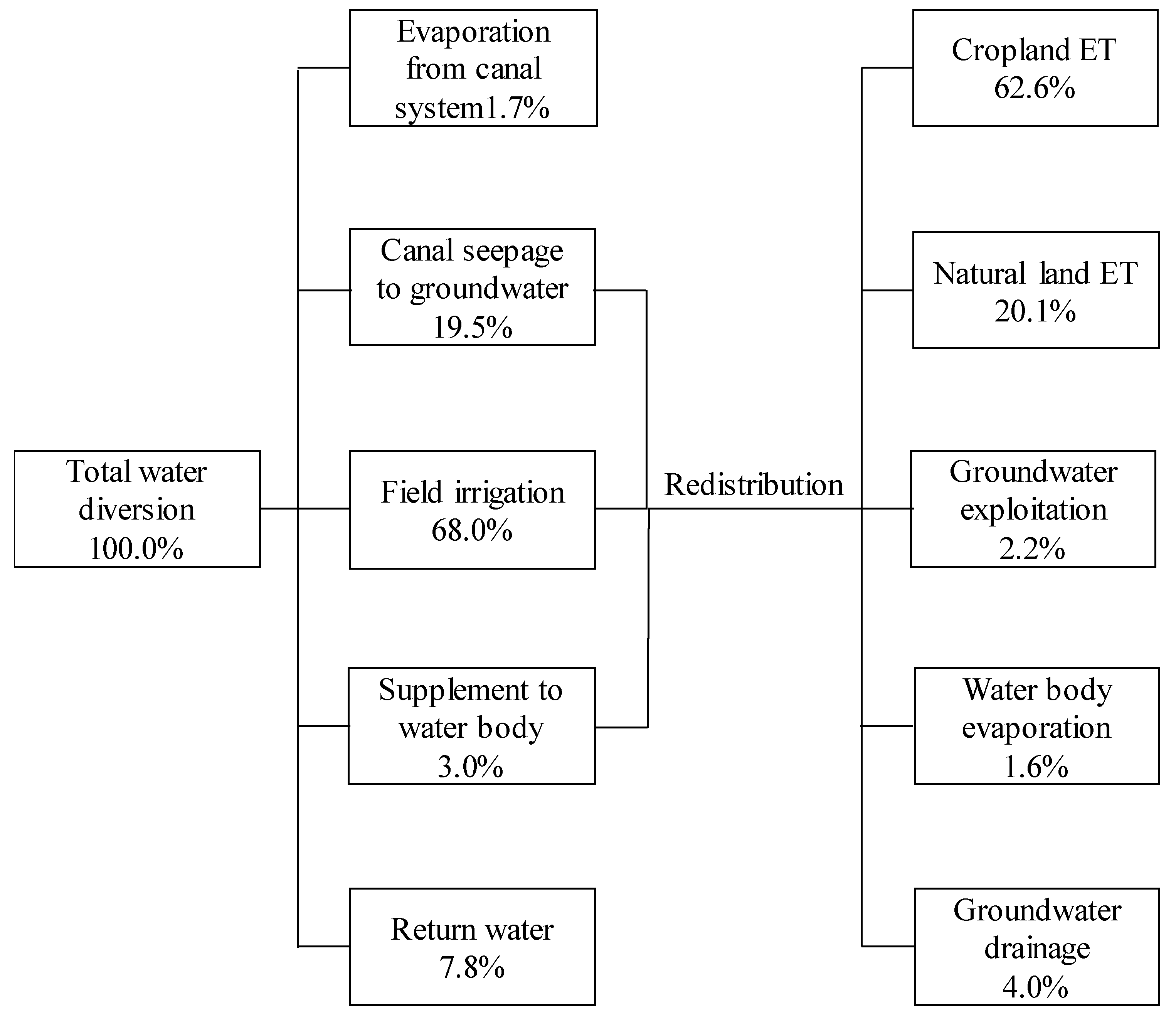
Irrigation was only applied to some of the crop fields during a water diversion. The uneven field percolation and canal seepage can trigger significant lateral groundwater flow, due to the local hydraulic gradients. Thus, the irrigation water was redistributed by the shallow groundwater system to some extent. As shown in Figure 6, assuming the total water diversion was 100%, then the evaporation from the canal system only accounted for about 1.7%, whereas the abandoned and return water that directly flow to the drainage systems were about 7.8%. These waters left the study area permanently. The water that recharged to the groundwater through canal seepage (19.5%), irrigated to the cropland (68.0%) and supplied to the water body (3.0%), remained in Jiyuan to continue their migration and transformation. Due to the site-specific water consumption ability and the well groundwater hydraulic connection, the remaining portions of water was redistributed by the shallow groundwater system, and eventually consumed by different land use types. Assuming precipitation was evapotranspirated preferentially, the proportion of diversion water that discharged through different pathways was calculated, and is shown in Figure 6. The cropland ET accounted for 62.6% of the diverted water, and was smaller than the irrigation water applied to cropland (68.0%), indicating that some water was transferred to other places. About 20.1% of the diverted water was consumed by ET of the natural land, even though no irrigation events occurred on this type of land. This part of water should mostly be contributed by canal seepage (Figure 6). The residential land consumed 2.2% of the diverted water through groundwater exploitation. Groundwater drainage accounted for 4% of the diverted water. Almost no irrigation water was consumed by the sand dune. The redistribution of irrigation water can benefit other crops and natural vegetation.
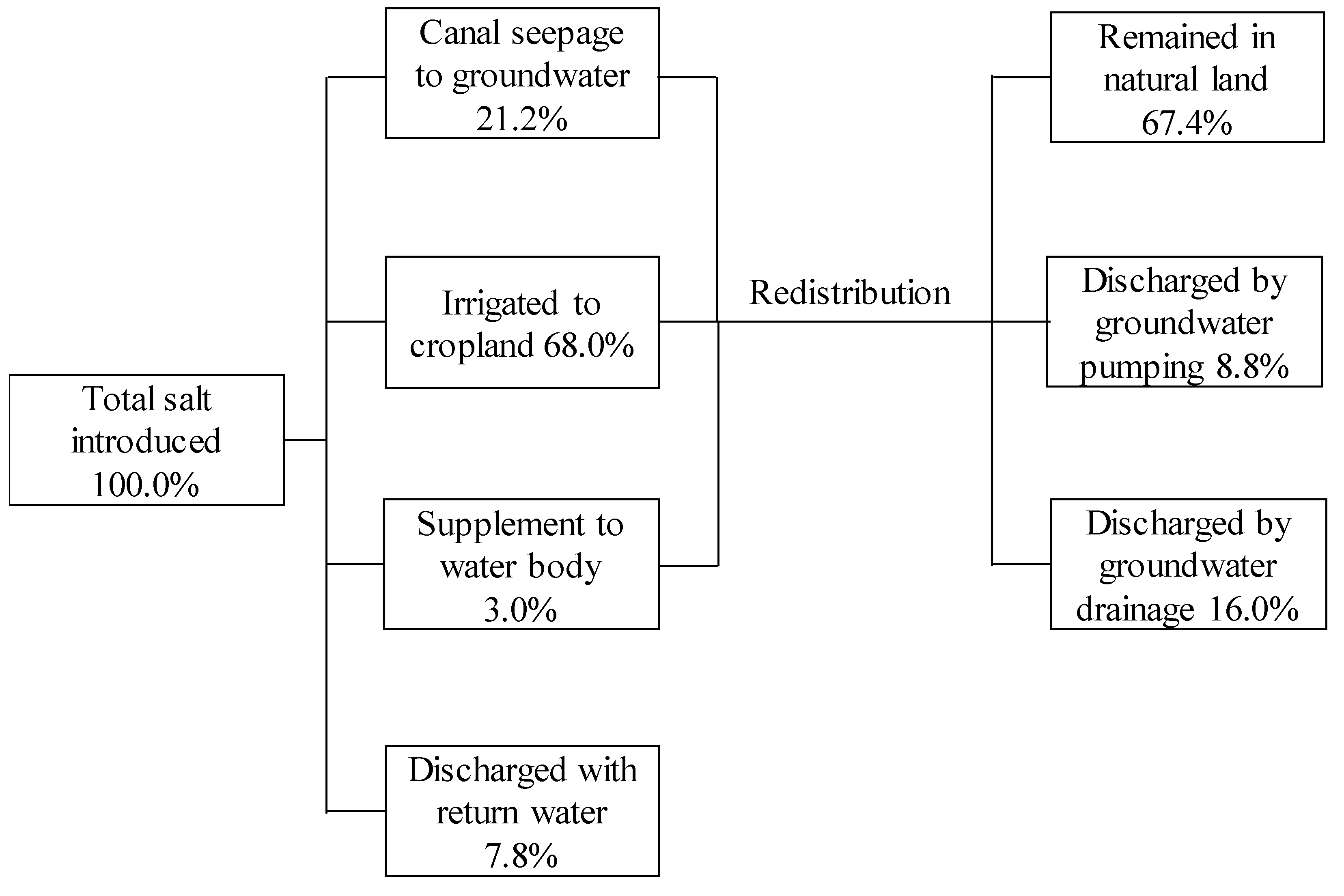
Along with the water, the salt that was introduced by irrigation water was also redistributed. Figure 7 shows that the total salt introduced (100.0%) was distributed to the cropland (68.0%), water body (3.0%), recharged to the groundwater through canal seepage (21.2%), and discharged with the return water (7.8%) in the first distribution. Except for the discharged salt, the other salt remained in the area, and began its secondary distribution through groundwater. The average total dissolved salt (TDS, g L−1) of diversion water was about 0.52 g L−1, while the TDS of groundwater in Jiyuan is about 2.1 g L−1. The TDS of precipitation and evapotranspiration is close to 0. Then, based on the water balance, the salt balance of different land use patterns can also be calculated by multiplying the water budgets by their TDS. Finally, the net salt accumulation of a given land use type and its proportion to the total salt introduced by irrigation water can be obtained. Results showed that after redistribution, the salt in the cropland, water body and sand dune did not increase (or even reduced), while the salt accumulation in the natural land accounted for 67.4% of the total introduced salt, the salt discharged by groundwater exploitation accounted for 8.8%, and that discharged with the drainage water accounted for 16.0% (Figure 7).
3.3.3. Salt Accumulation and Drainage
The shallow groundwater system may threaten crop production due to soil salinization and waterlogging problems [12]. As shown in Table 4, the shallow groundwater system backed up and stored the excess irrigation water, and especially during the non-growing season, the water stored by shallow groundwater was more than 50% of the water applied. If there were no shallow groundwaters, these waters would percolate thoroughly, with significant salt leaching effects. However, the real leaching effect was very low, and most of the leached salts could not be thoroughly discharged and remained in the deeper soil layers because of the shallow groundwater and poor field drainage systems. After that, salts migrated again with the upward water movement due to high evapotranspiration rates, and ended up reaccumulating in the upper layers [28]. Waterlogging problems also frequently occurred in the low lands, especially after a heavy irrigation or large rainfall events.
However, the shallow groundwater also provides the possibility for salt draining out of the irrigation districts through the shallow drainage systems, especially during the autumn irrigation period. Even though the salt drained out of the study area accounts for no more than 1/3 of the total salt introduced (Figure 7), most of the soluble Na+, which is harmful to soil [45] and crops, could be drained out effectively (referred to Akae et al. [46] and Liu et al. [47]). This may be the reason that the sodium balance of the whole district is almost stable at present [46], and thus, the actual salinization status of the district is better than stated by the traditional viewpoint. Without the shallow groundwater system, the drainage ditches will lose their ability to drain the soluble salts, and salt can only be leached to the deeper layers. Thus, they may continue to constitute a long-term hazard.
4. Conclusions
The shallow groundwater system plays a multifaceted role in arid irrigated agro-ecosystems. To clarify the role of shallow groundwater in an irrigation system (Jiyuan) located in the upper Yellow River basin, the year-round, growing season, and non-growing season water balance calculations were conducted for different land use types. Results showed that the shallow groundwater performed its functions in water storage and supply, water and salt redistribution, salt accumulation and drainage. About 36% of the total water applied during the year was temporarily stored in groundwater for further distribution. More than 90% of these waters was eventually re-consumed by evapotranspiration. Through redistribution, about 20% of the total diverted water migrated to the natural land, which accounted for about 70% of the natural land ET. As a result, 67% of the salt introduced by irrigation water accumulated in natural land, and the rest was discharged from the region. In this way, the salt in the cropland was not increased, or even reduced. However, the natural land suffered serious salinity problems due to salt accumulation [29]. The shallow groundwater system causes soil salinization on one hand, but provides the pathway for draining out some harmful ions on the other.
This study presents the advantages and disadvantages of the shallow groundwater system. To maintain the sustainability of the agroecosystem, the positive effects of shallow groundwaters should be retained, while the negative effects should be avoided. To achieve this, some practical measures are now suggested: (1) increasing the depth and density of drainage ditches, as well as using controlled drainage; (2) adding a leaching irrigation to the natural land to sustain natural vegetation; (3) promoting the conjunctive use of ground and surface water for irrigation in the areas with good groundwater quality.
Author Contributions
D.R., X.X. and G.H. conceived and designed this research. D.R. performed the field experiment, analyzed the data, and wrote the manuscript. X.X. and G.H. modified and improved the manuscript. Q.H., Z.H. and Y.X. made significant suggestions in data analysis and manuscript writing.
Acknowledgments
This research was jointly supported by the National Science Foundation of China (grant numbers: 51639009, 51679235 and 51125036), the 13th Five-year National Key Research and Development Program of the Chinese Ministry of Science and Technology (grant numbers: 2017YFC0403301).
Conflicts of Interest
The authors declare no conflict of interest.
References
- Northey, J.E.; Christen, E.W.; Ayars, J.E.; Jankowski, J. Occurrence and measurement of salinity stratification in shallow groundwater in the Murrumbidgee Irrigation Area, south-eastern Australia. Agric. Water Manag. 2006, 81, 23–40. [Google Scholar] [CrossRef]
- Pereira, L.S.; Gonçalves, J.M.; Dong, B.; Mao, Z.; Fang, S.X. Assessing basin irrigation and scheduling strategies for saving irrigation water and controlling salinity in the Upper Yellow River Basin, China. Agric. Water Manag. 2007, 93, 109–122. [Google Scholar] [CrossRef]
- Luo, Y.; Sophocleous, M. Seasonal groundwater contribution to crop-water use assessed with lysimeter observations and model simulations. J. Hydrol. 2010, 389, 325–335. [Google Scholar] [CrossRef]
- Karimov, A.K.; Šimůnek, J.; Hanjra, M.A.; Avliyakulov, M.; Forkutsa, I. Effects of the shallow water table on water use of winter wheat and ecosystem health: Implications for unlocking the potential of groundwater in the Fergana Valley (Central Asia). Agric. Water Manag. 2014, 131, 57–69. [Google Scholar] [CrossRef]
- Schmitter, P.; Zwart, S.J.; Danvi, A.; Gbaguidi, F. Contributions of lateral flow and groundwater to the spatio-temporal variation of irrigated rice yields and water productivity in a West-African inland valley. Agric. Water Manag. 2015, 152, 286–298. [Google Scholar] [CrossRef]
- Ayars, J.E.; Christen, E.W.; Hornbuckle, J.W. Controlled drainage for improved water management in arid regions irrigated agriculture. Agric. Water Manag. 2006, 86, 128–139. [Google Scholar] [CrossRef]
- Christen, E.W.; Ayars, J.E.; Hornbuckle, J.W. Subsurface drainage design and management in irrigated areas of Australia. Irrig. Sci. 2001, 21, 35–43. [Google Scholar] [CrossRef]
- Singh, A.; Krause, P.; Panda, S.N.; Flugel, W.A. Rising water table: A threat to sustainable agriculture in an irrigated semi-arid region of Haryana, India. Agric. Water Manag. 2010, 97, 1443–1451. [Google Scholar] [CrossRef]
- Nosetto, M.D.; Jobbágy, E.G.; Jackson, R.B.; Sznaider, G.A. Reciprocal influence of crops and shallow ground water in sandy landscapes of the Inland Pampas. Field Crops Res. 2009, 113, 138–148. [Google Scholar] [CrossRef]
- Ayars, J.E.; Christen, E.W.; Soppe, R.W.; Meyer, W.S. The resource potential of in-situ shallow ground water use in irrigated agriculture: A review. Irrig. Sci. 2006, 24, 147–160. [Google Scholar] [CrossRef]
- Kahlown, M.A.; Ashra, M.; Zia-ul-Haq. Effect of shallow groundwater table on crop water requirements and crop yields. Agric. Water Manag. 2005, 11, 24–35. [Google Scholar] [CrossRef]
- Ren, D.; Xu, X.; Engel, B.; Huang, G. Growth responses of crops and natural vegetation to irrigation and water table changes in an agro-ecosystem of Hetao, upper Yellow River basin: Scenario analysis on maize, sunflower, watermelon and tamarisk. Agric. Water Manag. 2018, 199, 93–104. [Google Scholar] [CrossRef]
- Šimůnek, J.; van Genuchten, M.T.; Šejna, M. Recent developments and applications of the HYDRUS computer software packages. Vadose Zone J. 2016, 15, 1–25. [Google Scholar] [CrossRef]
- Van Dam, J.C.; Groenendijk, P.; Hendriks, R.F.; Kroes, J.G. Advances of modeling water flow in variably saturated soils with SWAP. Vadose Zone J. 2008, 7, 640–653. [Google Scholar] [CrossRef]
- Harbaugh, A.W.; Banta, E.R.; Hill, M.C.; McDonald, M.G. MODFLOW-2000, the US Geological Survey Modular Groundwater Mode–User Guide to Modularization Concepts and the Groundwater Flow Process; Open-File Report 00-92; US Geological Survey: Reston, VA, USA, 2000. Available online: https://pubs.usgs.gov/of/2000/0092/report.pdf (accessed on 6 May 2018).
- Trefry, M.G.; Muffels, C. FEFLOW: A finite-element ground water flow and transport modeling tool. Groundwater 2007, 45, 525–528. [Google Scholar] [CrossRef]
- Hooghoudt, S.B. Waarnemingen van Grondwaterstanden Voor de Landbouw; Scientific Report [in Dutch]; Verslagen Technische Bijeenkomste; Commissie voor Hydrologisch TNO: The Hague, The Netherlands, 1952; Volume 1–6, pp. 94–110. [Google Scholar]
- Gillham, R.W. The capillary fringe and its effect on water-table response. J. Hydrol. 1984, 67, 307–324. [Google Scholar] [CrossRef]
- Weeks, E.P. The Lisse effect revisited. Groundwater 2002, 40, 652–656. [Google Scholar] [CrossRef]
- Appels, W.M.; Bogaart, P.W.; van der Zee, S.E.A.T.M. Feedbacks between Shallow Groundwater Dynamics and Surface Topography on Runoff Generation in Flat Fields. Water Resour. Res. 2017, 53, 10336–10353. [Google Scholar] [CrossRef]
- Abdulrazzak, M.J.; Sorman, A.U.; Alhames, A.S. Water balance approach under extreme arid conditions—A case study of Tabalah Basin, Saudi Arabia. Hydrol. Processes 1989, 3, 107–122. [Google Scholar] [CrossRef]
- Scanlon, B.R.; Healy, R.W.; Cook, P.G. Choosing appropriate techniques for quantifying groundwater recharge. Hydrogeol. J. 2002, 10, 18–39. [Google Scholar] [CrossRef]
- Xu, X.; Huang, G.H.; Qu, Z.Y.; Pereira, L.S. Assessing the groundwater dynamics and predicting impacts of water saving in the Hetao Irrigation District, Yellow River basin. Agric. Water Manag. 2010, 98, 301–313. [Google Scholar] [CrossRef]
- Machiwal, D.; Jha, M.K. GIS-based water balance modeling for estimating regional specific yield and distributed recharge in data-scarce hard-rock regions. J. Hydro-Environ. Res. 2015, 9, 554–568. [Google Scholar] [CrossRef]
- Xu, X.; Huang, G.H.; Qu, Z.Y.; Pereira, L.S. Using MODFLOW and GIS to assess changes in groundwater dynamics in response to water saving measures in irrigation districts of the upper Yellow River basin. Water Resour. Manag. 2011, 25, 2035–2059. [Google Scholar] [CrossRef]
- Miao, Q.; Shi, H.; Gonçalves, J.M.; Pereira, L.S. Field assessment of basin irrigation performance and water saving in Hetao, Yellow River basin: Issues to support irrigation systems modernisation. Biosyst. Eng. 2015, 136, 102–116. [Google Scholar] [CrossRef]
- Miao, Q.; Shi, H.; Gonçalves, J.M.; Pereira, L.S. Basin Irrigation Design with Multi-Criteria Analysis Focusing on Water Saving and Economic Returns: Application to Wheat in Hetao, Yellow River Basin. Water 2018, 10, 67. [Google Scholar] [CrossRef]
- Ren, D.; Xu, X.; Hao, Y.; Huang, G. Modeling and assessing field irrigation water use in a canal system of Hetao, upper Yellow River basin: Application to maize, sunflower and watermelon. J. Hydrol. 2016, 532, 122–139. [Google Scholar] [CrossRef]
- Ren, D.; Xu, X.; Ramos, T.B.; Huang, Q.; Huo, Z.; Huang, G. Modeling and assessing the function and sustainability of natural patches in salt-affected agro-ecosystems: Application to Tamarisk (Tamarix chinensis Lour.) in Hetao, upper Yellow River basin. J. Hydrol. 2017, 552, 490–504. [Google Scholar] [CrossRef]
- Gonçalves, J.M.; Pereira, L.S.; Fang, S.X.; Dong, B. Modelling and multicriteria analysis of water saving scenarios for an irrigation district in the upper Yellow River Basin. Agric. Water Manag. 2007, 94, 93–108. [Google Scholar] [CrossRef]
- Yu, B.; Jiang, L.; Shang, S. Dry drainage effect of Hetao irrigation district based on remote sensing evapotranspiration. Trans. CSAE 2016, 32, 1–8. (In Chinese) [Google Scholar]
- Allen, R.G.; Pereira, L.S.; Raes, D.; Smith, M. Crop Evapotranspiration: Guidelines for Computing Crop Water Requirements; FAO Irrigation and Drainage Paper No. 56; FAO: Rome, Italy, 1998. [Google Scholar]
- Sophocleous, M. The Role of Specific Yield in Ground-Water Recharge Estimations: A Numerical Study. Groundwater 1985, 23, 52–58. [Google Scholar] [CrossRef]
- Wang, L.P.; Chen, Y.X.; Zeng, G.F. Irrigation, Drainage and Salinization Control in Hetao Irrigation District of Inner Mongolia; Water Resources and Hydraulic Power Publisher: Beijing, China, 1993. (In Chinese) [Google Scholar]
- Jia, S.; Yue, W.; Wang, J. Groundwater balance in the Yichang irrigation sub-district in Inner Mongolia in the past 20 years. J. Beijing Norm. Univ. 2013, 49, 243–245. (In Chinese) [Google Scholar]
- Miao, Q.; Rosa, R.D.; Shi, H.; Paredes, P.; Zhu, L.; Dai, J.; Pereira, L.S. Modeling water use, transpiration and soil evaporation of spring wheat–maize and spring wheat–sunflower relay intercropping using the dual crop coefficient approach. Agric. Water Manag. 2016, 165, 211–229. [Google Scholar] [CrossRef]
- Wang, Z.; Zhao, X.; Wu, P.; Chen, X. Effects of water limitation on yield advantage and water use in wheat (Triticum aestivum L.)/maize (Zea mays L.) strip intercropping. Eur. J. Agron. 2015, 71, 149–159. [Google Scholar] [CrossRef]
- Hong, M.; Zeng, W.; Ma, T.; Lei, G.; Zha, Y.; Fang, Y.; Huang, J. Determination of growth stage-specific crop coefficients (kc) of sunflowers (Helianthus annuus L.) under salt stress. Water 2017, 9, 215. [Google Scholar]
- Lei, T.; Xiao, J.; Li, G.; Mao, J.; Wang, J.; Liu, Z.; Zhang, J. Effect of drip irrigation with saline water on water use efficiency and quality of watermelons. Water Resour. Manag. 2003, 17, 395–408. [Google Scholar]
- Zhang, H.; Xiong, Y.; Huang, G.; Xu, X.; Huang, Q. Effects of water stress on processing tomatoes yield, quality and water use efficiency with plastic mulched drip irrigation in sandy soil of the Hetao Irrigation District. Agric. Water Manag. 2017, 179, 205–214. [Google Scholar] [CrossRef]
- Yang, Y.; Shang, S.; Jiang, L. Remote sensing temporal and spatial patterns of evapotranspiration and the responses to water management in a large irrigation district of North China. Agric. For. Meteorol. 2012, 164, 112–122. [Google Scholar] [CrossRef]
- Bai, L.; Cai, J.; Liu, Y.; Chen, H.; Zhang, B.; Huang, L. Responses of field evapotranspiration to the changes of cropping pattern and groundwater depth in large irrigation district of Yellow River basin. Agric. Water Manag. 2017, 188, 1–11. [Google Scholar] [CrossRef]
- Yue, W.; Yang, J.; Tong, J.; Gao, H. Transfer and balance of water and salt in irrigation district of arid region. J. Hydraul. Eng. 2008, 39, 623–632. (In Chinese) [Google Scholar]
- Barros, R.; Isidoro, D.; Aragüés, R. Long-term water balances in La Violada irrigation district (Spain): I. Sequential assessment and minimization of closing errors. Agric. Water Manag. 2011, 102, 35–45. [Google Scholar] [CrossRef] [Green Version]
- Van der Zee, S.E.A.T.M.; Shah, S.H.H.; Vervoort, R.W. Root zone salinity and sodicity under seasonal rainfall due to feedback of decreasing hydraulic conductivity. Water Resour. Res. 2014, 50, 9432–9446. [Google Scholar] [CrossRef]
- Akae, T.; Nakao, C.; Shi, H.; Zhang, Y. Changes in the cations composition of water from irrigation to drainage and leaching requirement of the Hetao Irrigation District, Inner Mongolia. Trans. JSIDRE 2008, 253, 27–33. [Google Scholar]
- Liu, X.; Wang, L.; Zhang, S.; Zhang, Y. Evaluation of irrigation and drainage water cation composition and salt leaching requirement in Hetao Irrigation District. Chin. J. Eco-Agric. 2011, 19, 500–505. (In Chinese) [Google Scholar] [CrossRef]
Figure 1.
Location of the Hetao, Jiyuan Irrigation System (Jiyuan) and the observation points.

Figure 2.
Mean vegetation calendar of Jiyuan. The initial period of wheat (in April) was not shown.

Figure 3.
The amount of precipitation and year-round water diversion (6 to 7 times) to Jiyuan, from 2001 to 2013.
Figure 3.
The amount of precipitation and year-round water diversion (6 to 7 times) to Jiyuan, from 2001 to 2013.

Figure 4.
Spatially averaged groundwater depth fluctuations in Jiyuan from 2007 to 2010, compared with daily precipitation and irrigation depths.
Figure 4.
Spatially averaged groundwater depth fluctuations in Jiyuan from 2007 to 2010, compared with daily precipitation and irrigation depths.

Figure 5.
The Annual ETO during the growing season (May to September) and non-growing season, from 2001 to 2013.
Figure 5.
The Annual ETO during the growing season (May to September) and non-growing season, from 2001 to 2013.

Figure 6.
The consumption pathway of diversion water in Jiyuan.

Figure 7.
The discharge and redistribution of the introduced salt by water diversion in Jiyuan.


Table 1.
Range of irrigation depths observed at Jiyuan during the growing season in 2012 and 2013.
| Irrigation Event | Year | Date (Month/Day) | Crop | Irrigation Depth (mm) | Year | Date (Month/Day) | Crop | Irrigation Depth (mm) |
|---|---|---|---|---|---|---|---|---|
| First | 2012 | 05/02–05/07 | Sunflower | 150–206 | 2013 | 05/10–05/14 | Sunflower | 162–223 |
| Wheat | 108–149 | Wheat | 64–88 | |||||
| Vegetable | 150–206 | Vegetable | 151–208 | |||||
| Second | 05/23–05/27 | Wheat | 63–87 | 05/25 | Wheat | 62–86 | ||
| Third | 06/22–06/26 | Maize | 94–129 | 06/25–07/01 | Maize | 90–123 | ||
| Sunflower | 72–99 | Sunflower | 82–113 | |||||
| Wheat | 61–84 | Wheat | 59–81 | |||||
| Fourth | 08/02–08/04 | Maize | 91–125 | 07/15–07/19 | Maize | 75–103 | ||
| Sunflower | 74–101 | Sunflower | 85–117 | |||||
| Fifth | 08/28–09/01 | Maize | 60–83 | 08/06–08/10 | Maize | 86–119 | ||
| Sunflower | 72–99 |
Table 2.
Year-round and growing season (May to September) evapotranspiration for the whole Jiyuan (ET), cropland(ETC), natural land (ETN), residential land (ETR), sand dune (ETS) and water body (ETW).
Table 2.
Year-round and growing season (May to September) evapotranspiration for the whole Jiyuan (ET), cropland(ETC), natural land (ETN), residential land (ETR), sand dune (ETS) and water body (ETW).
| Year | Year-Round Evapotranspiration (mm) | Growing Season Evapotranspiration (mm) | ||||||||||
|---|---|---|---|---|---|---|---|---|---|---|---|---|
| ET | ETC | ETN | ETR | ETS | ETW | ET | ETC | ETN | ETR | ETS | ETW | |
| 2001 | 559 | 638 | 490 | 159 | 143 | 1282 | 444 | 512 | 376 | 150 | 135 | 884 |
| 2002 | 594 | 685 | 515 | 148 | 134 | 1343 | 461 | 532 | 399 | 126 | 113 | 899 |
| 2003 | 611 | 712 | 517 | 140 | 126 | 1356 | 452 | 510 | 412 | 126 | 113 | 925 |
| 2004 | 626 | 739 | 508 | 161 | 145 | 1271 | 477 | 557 | 399 | 147 | 132 | 826 |
| 2005 | 656 | 777 | 553 | 77 | 69 | 1316 | 437 | 512 | 372 | 72 | 65 | 899 |
| 2006 | 622 | 748 | 474 | 175 | 158 | 1251 | 466 | 560 | 350 | 162 | 146 | 836 |
| 2007 | 584 | 684 | 478 | 166 | 149 | 1420 | 433 | 511 | 349 | 123 | 110 | 983 |
| 2008 | 650 | 744 | 568 | 201 | 181 | 1221 | 498 | 567 | 435 | 182 | 164 | 827 |
| 2009 | 628 | 766 | 482 | 88 | 79 | 1327 | 485 | 595 | 364 | 78 | 70 | 902 |
| 2010 | 686 | 807 | 574 | 136 | 123 | 1402 | 508 | 589 | 440 | 131 | 118 | 937 |
| 2011 | 663 | 796 | 545 | 47 | 42 | 1413 | 418 | 498 | 346 | 40 | 36 | 964 |
| 2012 | 712 | 815 | 626 | 208 | 187 | 1355 | 499 | 570 | 428 | 203 | 183 | 894 |
| 2013 | 580 | 676 | 497 | 104 | 94 | 1427 | 438 | 501 | 391 | 103 | 93 | 920 |
| Average | 628 | 737 | 525 | 139 | 125 | 1337 | 463 | 539 | 389 | 126 | 114 | 900 |
Table 3.
Lateral groundwater exchanges of the different land use types. These data can be converted to volume amount (m3), based on the area of different land use types, as described in Part 2.1.
Table 3.
Lateral groundwater exchanges of the different land use types. These data can be converted to volume amount (m3), based on the area of different land use types, as described in Part 2.1.
| Year | Year−Round Lateral Groundwater Exchange (mm) | Growing Season Lateral Groundwater Exchange (mm) | ||||||||
|---|---|---|---|---|---|---|---|---|---|---|
| QC | QN | QR | QS | QW | QC | QN | QR | QS | QW | |
| 2001 | −203 | 323 | 148 | −20 | −1177 | −74 | 195 | 51 | −42 | −1067 |
| 2002 | −242 | 369 | 181 | −6 | −1105 | −99 | 236 | 56 | −46 | −1027 |
| 2003 | −182 | 351 | 168 | −25 | −1085 | −73 | 237 | 49 | −53 | −1001 |
| 2004 | −219 | 351 | 218 | 4 | −1190 | −105 | 214 | 74 | −42 | −1122 |
| 2005 | −201 | 434 | 192 | −28 | −1061 | −76 | 252 | 71 | −46 | −973 |
| 2006 | −217 | 310 | 260 | 6 | −1225 | −90 | 160 | 100 | −37 | −1126 |
| 2007 | −230 | 322 | 274 | 3 | −1046 | −110 | 177 | 86 | −55 | −939 |
| 2008 | −229 | 363 | 277 | −14 | −1280 | −78 | 212 | 102 | −57 | −1155 |
| 2009 | −223 | 384 | 295 | 2 | −1061 | −85 | 207 | 77 | −78 | −976 |
| 2010 | −265 | 438 | 325 | 8 | −1034 | −127 | 249 | 105 | −64 | −994 |
| 2011 | −243 | 472 | 317 | −3 | −934 | −107 | 275 | 143 | −23 | −877 |
| 2012 | −195 | 379 | 313 | −43 | −1153 | −61 | 191 | 143 | −48 | −1109 |
| 2013 | −252 | 397 | 377 | 15 | −977 | −134 | 231 | 131 | −58 | −983 |
| Average | −223 | 376 | 257 | −8 | −1102 | −94 | 218 | 91 | −50 | −1027 |
Note: a positive value indicates a net inflow to the land use type, while a negative value means a net outflow.
Table 4.
Temporary water storage of the shallow groundwater system.
| Year | Year-Round | Growing Season | Non-Growing Season | ||||||
|---|---|---|---|---|---|---|---|---|---|
| Water Application (mm) | Water Storage (mm) | Ratio of Water Storage to Water Application | Water Application (mm) | Water Storage (mm) | Ratio of Water Storage to Water Application | Water Application (mm) | Water Storage (mm) | Ratio of Water Storage to Water Application | |
| 2001 | 640 | 262 | 0.41 | 439 | 138 | 0.31 | 200 | 123 | 0.62 |
| 2002 | 706 | 243 | 0.34 | 460 | 109 | 0.24 | 245 | 134 | 0.55 |
| 2003 | 660 | 263 | 0.40 | 417 | 108 | 0.26 | 244 | 155 | 0.64 |
| 2004 | 734 | 283 | 0.39 | 489 | 127 | 0.26 | 245 | 156 | 0.64 |
| 2005 | 691 | 278 | 0.40 | 407 | 105 | 0.26 | 284 | 173 | 0.61 |
| 2006 | 747 | 253 | 0.34 | 491 | 111 | 0.23 | 256 | 142 | 0.56 |
| 2007 | 708 | 225 | 0.32 | 444 | 148 | 0.33 | 264 | 77 | 0.29 |
| 2008 | 749 | 256 | 0.34 | 484 | 110 | 0.23 | 265 | 146 | 0.55 |
| 2009 | 725 | 233 | 0.32 | 451 | 107 | 0.24 | 274 | 126 | 0.46 |
| 2010 | 805 | 242 | 0.30 | 506 | 124 | 0.25 | 300 | 118 | 0.39 |
| 2011 | 738 | 271 | 0.37 | 422 | 138 | 0.33 | 316 | 133 | 0.42 |
| 2012 | 754 | 274 | 0.36 | 485 | 135 | 0.28 | 269 | 138 | 0.51 |
| 2013 | 697 | 291 | 0.42 | 442 | 148 | 0.33 | 255 | 144 | 0.56 |
| Average | 720 | 260 | 0.36 | 457 | 124 | 0.27 | 263 | 136 | 0.52 |
Note: Water application including water diversion (I) and precipitation (P).
© 2018 by the authors. Licensee MDPI, Basel, Switzerland. This article is an open access article distributed under the terms and conditions of the Creative Commons Attribution (CC BY) license (http://creativecommons.org/licenses/by/4.0/).
Share and Cite
MDPI and ACS Style
Ren, D.; Xu, X.; Huang, Q.; Huo, Z.; Xiong, Y.; Huang, G. Analyzing the Role of Shallow Groundwater Systems in the Water Use of Different Land-Use Types in Arid Irrigated Regions. Water 2018, 10, 634. https://doi.org/10.3390/w10050634
AMA Style
Ren D, Xu X, Huang Q, Huo Z, Xiong Y, Huang G. Analyzing the Role of Shallow Groundwater Systems in the Water Use of Different Land-Use Types in Arid Irrigated Regions. Water. 2018; 10(5):634. https://doi.org/10.3390/w10050634
Chicago/Turabian StyleRen, Dongyang, Xu Xu, Quanzhong Huang, Zailin Huo, Yunwu Xiong, and Guanhua Huang. 2018. "Analyzing the Role of Shallow Groundwater Systems in the Water Use of Different Land-Use Types in Arid Irrigated Regions" Water 10, no. 5: 634. https://doi.org/10.3390/w10050634
Note that from the first issue of 2016, this journal uses article numbers instead of page numbers. See further details here.